BERT: Pre-training of Deep Bidirectional Transformers for Language Understanding: Course

Learning Objectives

By the end of this course, you will be able to:

1. Explain why left-to-right language models fail on tasks that need context from both directions
2. Describe how BERT’s Transformer encoder differs from GPT’s Transformer decoder
3. Construct BERT’s three-part input representation (token + segment + position embeddings)
4. Walk through the masked language modeling procedure, including the 80/10/10 masking strategy
5. Compute BERT’s classification and question-answering outputs by hand using dot products and softmax
6. Explain how one pre-trained model adapts to classification, question answering, and token-level tasks with minimal new parameters

Prerequisites

• Python and numpy – you should be comfortable with functions, loops, and array operations
• Matrix multiplication and dot products – multiplying matrices and computing similarity between vectors
• Softmax function – converts raw scores into a probability distribution that sums to 1. Covered in the Transformer course.
• Cross-entropy loss – measures how well predicted probabilities match true labels: \(-\log P(\text{correct class})\)
• The Transformer architecture – multi-head self-attention, positional encodings, feed-forward layers, residual connections, and layer normalization. You should have completed the Transformer course (see Attention Is All You Need).
• The pre-train-then-fine-tune paradigm – the idea of training on unlabeled text first, then adapting to specific tasks. Covered in the GPT course (see Improving Language Understanding by Generative Pre-Training).

Lesson 1: The Limits of Left-to-Right

GPT showed that pre-training a Transformer on unlabeled text and then fine-tuning it on specific tasks was a powerful recipe. But GPT has a fundamental limitation: it reads text in only one direction. This lesson explains why that matters and what it costs.

Explanation

Imagine reading a mystery novel, but you are only allowed to read each sentence from left to right, one word at a time, without ever looking ahead. When you encounter the sentence “The bank by the river was muddy,” you read “The bank” and must form an understanding of “bank” before seeing “river.” You might picture a financial institution. Only when you reach “river” do you realize it meant a riverbank – but by then, your internal model of the sentence was built on the wrong interpretation.

A human reader does not have this problem. When we read, our eyes jump back and forth. We understand “bank” in the context of the whole sentence – “by the river” on the right tells us just as much as “The” on the left. We use bidirectional context.

GPT is stuck reading left-to-right. It uses the Transformer decoder with a causal attention mask: each token can only attend to tokens before it (see Improving Language Understanding by Generative Pre-Training). When GPT processes “bank” at position 2, it only sees [“The”, “bank”] – it cannot look ahead to “river” or “muddy.” This means GPT’s representation of “bank” is built on partial information.

An earlier approach, ELMo, tried to work around this by training two separate models: one left-to-right and one right-to-left. It then concatenated (glued together) their outputs. But this is shallow bidirectionality – the left-to-right model never actually sees right-to-left context during its own computation. It is like asking two people to each read half a book and then stapling their summaries together, rather than having one person read the whole book.

The cost of this limitation is measurable. On tasks where both directions matter – question answering, natural language inference, named entity recognition – left-to-right models underperform. Question answering is the clearest example: to answer “Where was the battle fought?” given a passage, the model needs to connect the question tokens with answer tokens that could appear anywhere in the passage. A left-to-right model processing the passage cannot look ahead to see if future tokens contain the answer.

BERT’s key insight: replace next-word prediction with fill-in-the-blank. Instead of predicting the next word (which requires a left-to-right constraint), mask out random words and predict them from context on both sides. This removes the need for a causal mask and allows every token to attend to every other token.

Worked Example

Consider the sentence: “The cat sat on the mat.”

GPT (left-to-right): When building the representation at position 3 (“on”), GPT’s attention can see:

The representation of “on” knows nothing about “the mat” that follows.

BERT (bidirectional): Every token attends to every other token. The representation at position 3 (“on”) sees:

BERT’s representation of “on” uses context from both sides simultaneously. This means “on” can directly interact with “mat” in the same attention layer, while GPT’s “on” must wait until “mat” has been processed (which never happens, because GPT processes left-to-right).

Now consider an ambiguous word: “The bank issued a statement.” vs. “The bank eroded during the flood.”

• In the first sentence, the right context “issued a statement” makes “bank” mean a financial institution.
• In the second, “eroded during the flood” makes “bank” mean a riverbank.

GPT must build its representation of “bank” before seeing the disambiguating context. BERT sees both sides at once and can build the correct representation from the start.

Exercises

Recall: What are the three approaches to reading direction that existed before BERT? (GPT, ELMo, and what BERT introduced.) Which is “deeply” bidirectional and why?

Apply: For the sentence “She picked up the light bag and the heavy suitcase,” explain what information is available to a left-to-right model at the word “light” vs. what a bidirectional model sees. How might this affect the model’s understanding of “light” (which could mean “not heavy” or “illumination”)?

Extend: If bidirectional context is so valuable, why can’t you simply train a standard language model bidirectionally? (Hint: think about what happens if a word can “see itself” through the network layers during prediction. The answer motivates the masking strategy in Lesson 4.)

Lesson 2: The Transformer Encoder

BERT uses the encoder half of the Transformer architecture. This lesson explains what “encoder-only” means, how it differs from GPT’s decoder-only architecture, and what BERT’s specific configuration looks like.

Explanation

Recall from the Transformer course that the original Transformer has two halves: an encoder that reads the full input with bidirectional attention, and a decoder that generates output one token at a time with masked (left-to-right) attention. GPT uses only the decoder. BERT makes the opposite choice: it uses only the encoder.

Think of it this way. The decoder is like a writer composing a sentence word by word – each word is chosen based on what came before. The encoder is like a reader taking in an entire paragraph at once, with every word informing the understanding of every other word. BERT is a reader, not a writer. It is designed to understand text, not generate it.

Concretely, the Transformer encoder block has the same components you learned in the Transformer course:

1. Multi-head self-attention – each token computes attention scores with every other token, with no masking (unlike GPT’s causal mask)
2. Feed-forward network – a two-layer neural network applied independently to each position
3. Residual connections and layer normalization – stabilize training

The key difference from GPT is in step 1: no causal mask. In BERT, the attention matrix is full – position \(i\) can attend to position \(j\) regardless of whether \(j\) comes before or after \(i\).

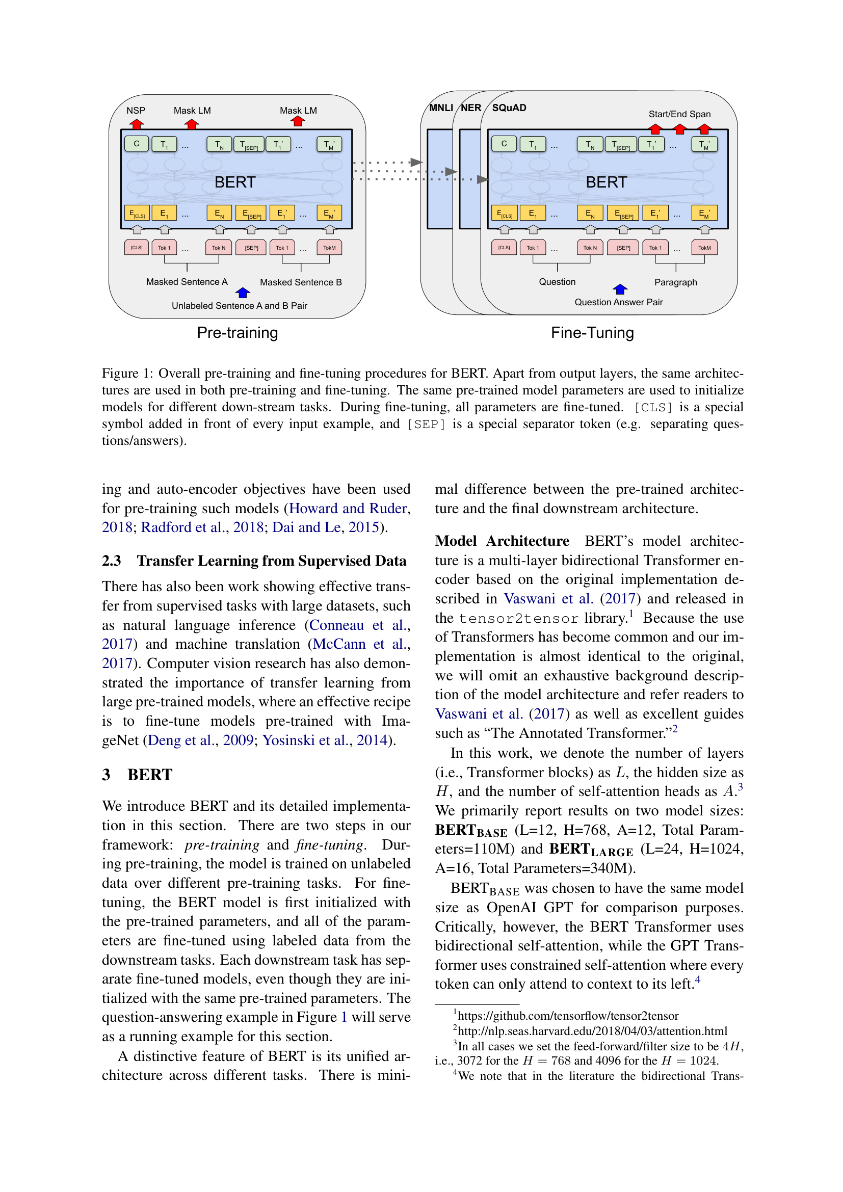
The paper’s Figure 1 shows the overall BERT framework. The same architecture is used for both pre-training and fine-tuning – only the output layer changes:

BERT defines two model sizes:

BERT_BASE was deliberately sized to match GPT (12 layers, 768 hidden, 110M parameters) so that any performance difference would come from the training approach, not the model size. The feed-forward size is always \(4H\) (3072 = 4 \(\times\) 768 for BERT_BASE, 4096 = 4 \(\times\) 1024 for BERT_LARGE).

Each attention head operates in a dimension of \(H / A\). For BERT_BASE: \(768 / 12 = 64\) dimensions per head. For BERT_LARGE: \(1024 / 16 = 64\) dimensions per head. The per-head dimension is the same in both models.

The paper also uses learned positional embeddings (like GPT) instead of the original Transformer’s sinusoidal encodings, and GELU (Gaussian Error Linear Unit – a smooth approximation to ReLU that allows small negative values through instead of zeroing them out) activation instead of ReLU in the feed-forward layers.

Worked Example

Let’s compare the attention patterns of BERT and GPT for a 4-token input: [“The”, “cat”, “is”, “cute”].

GPT’s attention mask (causal – lower triangular):

\[\text{Mask}_{\text{GPT}} = \begin{bmatrix} 1 & 0 & 0 & 0 \\ 1 & 1 & 0 & 0 \\ 1 & 1 & 1 & 0 \\ 1 & 1 & 1 & 1 \end{bmatrix}\]

“is” (row 2) can attend to “The”, “cat”, and “is” – but not “cute.”

BERT’s attention mask (full – no masking):

\[\text{Mask}_{\text{BERT}} = \begin{bmatrix} 1 & 1 & 1 & 1 \\ 1 & 1 & 1 & 1 \\ 1 & 1 & 1 & 1 \\ 1 & 1 & 1 & 1 \end{bmatrix}\]

Every position attends to every other position. “is” (row 2) attends to all four tokens, including “cute.”

Now let’s count the total attention connections across all 12 layers. For a sequence of length \(n\):

• GPT: Each layer has \(n(n+1)/2\) attention connections (triangular). For \(n = 512\): \(512 \times 513 / 2 = 131{,}328\) connections per layer.
• BERT: Each layer has \(n^2\) connections (full). For \(n = 512\): \(512^2 = 262{,}144\) connections per layer.

BERT has exactly twice as many attention connections per layer. This is the computational cost of bidirectionality – but also the source of its power.

Exercises

Recall: BERT uses the Transformer encoder; GPT uses the Transformer decoder. What is the single most important difference between them in terms of how attention works? Why does this difference exist?

Apply: BERT_BASE has 12 layers, each with a 768-dimensional feed-forward network that expands to 3072 dimensions. How many parameters are in the feed-forward networks across all 12 layers? (Each feed-forward layer has two weight matrices: \(W_1\) of shape \(768 \times 3072\) and \(W_2\) of shape \(3072 \times 768\), plus two bias vectors.)

Extend: BERT is an encoder-only model, which means it cannot generate text autoregressively (one token at a time). Why not? What architectural property of the encoder prevents autoregressive generation? (Hint: think about what information would leak if you tried to predict the next token using a bidirectional model.)

Lesson 3: Input Representation

Before BERT can process text, it needs to convert tokens into numbers. BERT uses a distinctive three-part input representation that handles both single sentences and sentence pairs. This lesson covers how inputs are constructed, including the special tokens that make BERT’s flexibility possible.

Explanation

Think of shipping a package. You need three labels: what is inside (the item name), which shipment it belongs to (batch number), and where it goes in the delivery sequence (position number). BERT labels each token with three analogous pieces of information, each encoded as a learned vector:

\[E_{\text{input}} = E_{\text{token}} + E_{\text{segment}} + E_{\text{position}}\]

• \(E_{\text{token}}\): a learned embedding for the specific word piece. BERT uses WordPiece tokenization with a vocabulary of 30,000 tokens. Common words like “the” get their own token; rare words are split into subwords (e.g., “playing” might become “play” + “##ing”, where “##” indicates a continuation).
• \(E_{\text{segment}}\): a learned embedding indicating whether this token belongs to sentence A or sentence B. There are only two segment embeddings (\(E_A\) and \(E_B\)), learned during pre-training.
• \(E_{\text{position}}\): a learned embedding encoding the token’s position in the sequence, from position 0 to position 511 (BERT supports sequences up to 512 tokens).

These three vectors are summed element-wise (not concatenated) to produce the final input representation for each token. All three have the same dimension \(H\) (768 for BERT_BASE).

BERT uses two special tokens:

• [CLS] (classification): always the first token of every input. Its final hidden state \(C \in \mathbb{R}^H\) serves as the aggregate representation of the entire input. For classification tasks, this is the vector that gets fed to the output layer.
• [SEP] (separator): marks the boundary between sentence A and sentence B. Also appears at the very end of the input.

For a single sentence like sentiment analysis:

[CLS] the film was great [SEP]

For a sentence pair like question answering:

[CLS] Where was the battle fought ? [SEP] The battle took place near the river . [SEP]

In the sentence pair case, all tokens from “Where” through the first “[SEP]” receive segment embedding \(E_A\), and all tokens from “The” through the second “[SEP]” receive segment embedding \(E_B\).

Worked Example

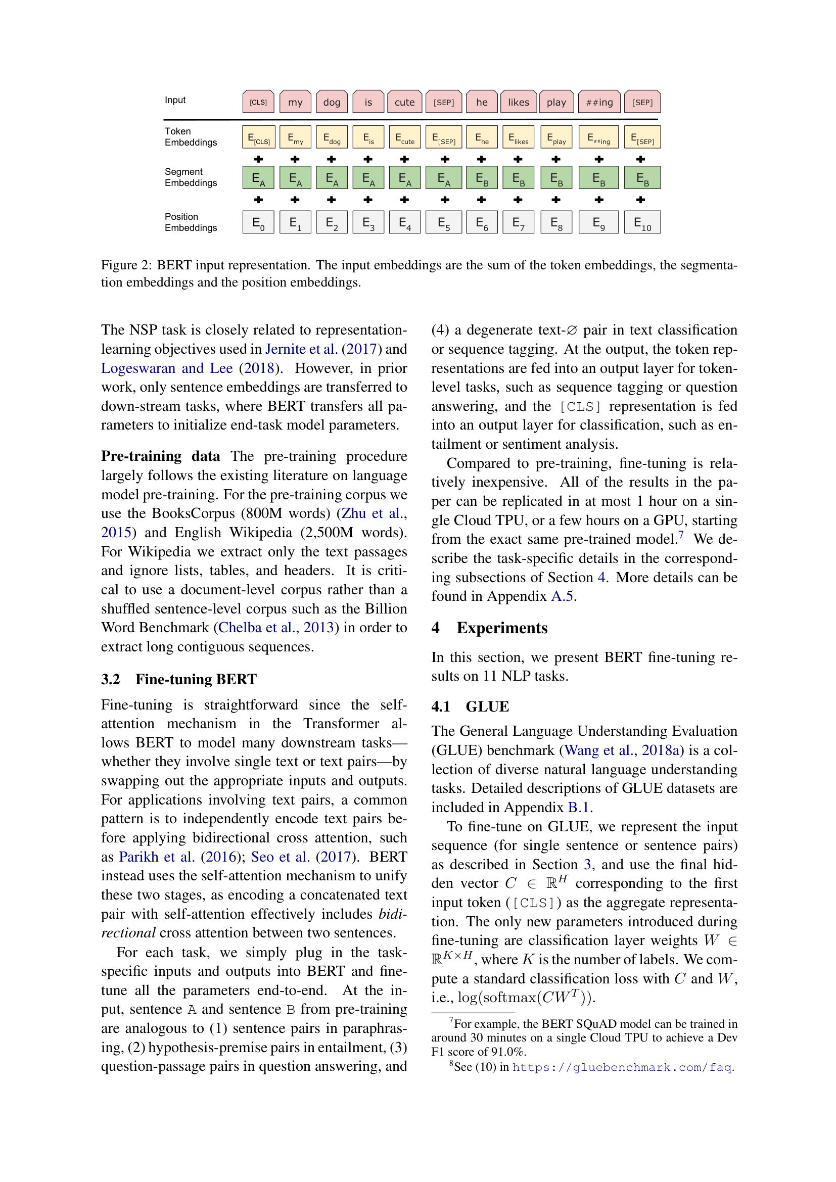
Let’s construct the input representation for the sentence pair: “my dog is cute [SEP] he likes play ##ing [SEP]”, preceded by [CLS].

The full token sequence is:

Now let’s compute the input embedding for one token using a tiny \(H = 4\) model.

For “dog” at position 2 in segment A:

\[E_{\text{token}}(\text{dog}) = [0.3, -0.5, 0.8, 0.1]\] \[E_{\text{segment}}(A) = [0.1, 0.2, -0.1, 0.0]\] \[E_{\text{position}}(2) = [0.0, -0.3, 0.2, 0.4]\]

\[E_{\text{input}} = [0.3 + 0.1 + 0.0, \; -0.5 + 0.2 + (-0.3), \; 0.8 + (-0.1) + 0.2, \; 0.1 + 0.0 + 0.4]\] \[= [0.4, -0.6, 0.9, 0.5]\]

For “he” at position 6 in segment B:

\[E_{\text{token}}(\text{he}) = [-0.2, 0.7, 0.4, -0.3]\] \[E_{\text{segment}}(B) = [-0.1, 0.3, 0.1, -0.2]\] \[E_{\text{position}}(6) = [0.5, 0.1, -0.4, 0.3]\]

\[E_{\text{input}} = [-0.2 + (-0.1) + 0.5, \; 0.7 + 0.3 + 0.1, \; 0.4 + 0.1 + (-0.4), \; -0.3 + (-0.2) + 0.3]\] \[= [0.2, 1.1, 0.1, -0.2]\]

Notice that “he” and “dog” start with different segment embeddings (\(E_B\) vs. \(E_A\)). This is how BERT tells them apart as belonging to different sentences, even though they are processed in the same sequence. The segment embedding difference (\(E_B - E_A = [-0.2, 0.1, 0.2, -0.2]\)) shifts all sentence-B tokens in a consistent direction in the embedding space.

Exercises

Recall: What are the three embedding types that BERT sums to create its input representation? Why does BERT sum them instead of concatenating them?

Apply: BERT_BASE has a vocabulary of 30,000 tokens, a maximum sequence length of 512, and a hidden size of 768. How many total parameters are in the three embedding tables (token embeddings + segment embeddings + position embeddings)? Which table is by far the largest?

Extend: GPT uses two embedding types (token + position) and handles sentence pairs by concatenating them with a [Delim] token. BERT adds segment embeddings as a third type. Why does BERT need segment embeddings when it already has [SEP] tokens as separators? (Hint: consider what information is available at each layer of the Transformer. Does a token 50 positions away from [SEP] know which sentence it belongs to without the segment embedding?)

Lesson 4: Masked Language Modeling

Masked language modeling is BERT’s core innovation – the training objective that makes bidirectional pre-training possible. This lesson explains how it works, why it works, and the clever 80/10/10 masking strategy that addresses the train-test mismatch.

Explanation

Imagine a language class where the teacher gives you sentences with blanks: “The cat ___ on the mat.” To fill in the blank, you naturally look at words on both sides – “cat” on the left and “on the mat” on the right. You consider the full context. This is fundamentally different from GPT’s training, where you predict the next word using only previous words.

BERT trains by playing this fill-in-the-blank game at massive scale. For each input sequence, BERT randomly selects 15% of the tokens for prediction. The model must predict the original token at each selected position, using context from both directions. This is called the Masked Language Model (MLM) objective, inspired by the Cloze task from a 1953 psychology study.

Why masking is necessary: You cannot simply train a bidirectional model to predict every token from its context. In a multi-layer network, if token \(i\) can attend to itself through the layers, it would trivially learn to copy its own input – the prediction becomes a lookup, not a reasoning task. By masking the target token, BERT forces the model to reconstruct it from surrounding context.

The masking procedure: For each training sequence, BERT chooses 15% of positions at random. Of those chosen positions:

• 80% of the time: replace the token with [MASK]. Example: “my dog is hairy” → “my dog is [MASK]”
• 10% of the time: replace the token with a random word from the vocabulary. Example: “my dog is hairy” → “my dog is apple”
• 10% of the time: keep the token unchanged. Example: “my dog is hairy” → “my dog is hairy”

In all three cases, the model must predict the original token (“hairy”).

Why the 80/10/10 split? This addresses a mismatch between pre-training and fine-tuning. During pre-training, the model sees [MASK] tokens. During fine-tuning, there are no [MASK] tokens – the model sees normal text. If the model only ever saw [MASK] during training, it might behave strangely on unmasked text during fine-tuning.

The 10% random replacement teaches the model that it cannot blindly trust the token at any position – it might be wrong. The 10% unchanged teaches the model to represent the actual token faithfully, since sometimes the “masked” position still contains the correct word. Together, these reduce the model’s dependence on the [MASK] token specifically.

Since only 15% of tokens are masked per sequence, the model only gets a training signal from 15% of positions per batch. This means BERT needs more training steps to converge compared to GPT (which gets a signal from every position). The BERT paper trained for 1 million steps – approximately 40 passes over the data.

Independence assumption: BERT predicts each masked token independently. If “New” and “York” are both masked in the same sentence, BERT predicts each without knowing what the other was predicted as. This is a limitation – it cannot model dependencies between masked positions.

Worked Example

Let’s trace the MLM procedure for the sentence: “the cat sat on the mat”.

Step 1: Select 15% of tokens for masking.

The sentence has 6 tokens. 15% of 6 is 0.9 – round to 1 token. Suppose position 3 (“on”) is selected.

Step 2: Apply the 80/10/10 replacement.

Draw a random number. Suppose we get 0.73, which falls in the 80% range (0.00-0.80):

• Replace “on” with [MASK]: “the cat sat [MASK] the mat”

Step 3: Process through BERT.

The 12-layer Transformer encoder processes all 6 tokens. Because attention is bidirectional, the [MASK] at position 3 attends to all other positions:

• Position 0 (“the”): context word
• Position 1 (“cat”): context word – a cat often sits on something
• Position 2 (“sat”): context word – “sat” strongly predicts a preposition follows
• Position 3 ([MASK]): the position to predict
• Position 4 (“the”): context word – an article follows, suggesting a noun phrase
• Position 5 (“mat”): context word – “mat” is a surface, suggesting “on” as the preposition

Step 4: Predict the masked token.

The model takes the final hidden vector \(T_3 \in \mathbb{R}^H\) at position 3 and projects it to a vocabulary-size vector using an output matrix, followed by softmax. Using a tiny vocabulary of 8 tokens:

Hidden vector: \(T_3 = [0.8, -0.3, 1.2, -0.5]\) (for \(H = 4\))

Suppose the output projection gives these logits (unnormalized scores before softmax) and probabilities:

Loss for this position: \(-\log P(\text{on}) = -\log(0.72) = 0.33\)

The model correctly assigns the highest probability to “on.” It uses both left context (“cat sat”) and right context (“the mat”) to make this prediction.

Step 5: Total MLM loss.

The loss is averaged over all masked positions in the batch. If we had masked 3 tokens across multiple sequences with losses 0.33, 0.85, and 1.21:

\[L_{\text{MLM}} = \frac{0.33 + 0.85 + 1.21}{3} = 0.797\]

Exercises

Recall: Why does BERT mask tokens instead of simply training a bidirectional model to predict every token? What problem would occur without masking?

Apply: A training sequence has 20 tokens. BERT selects 3 tokens for masking (15%). For each selected token, determine the replacement using these random draws: token 1 gets 0.42, token 2 gets 0.87, token 3 gets 0.95. What happens to each token? (Use the 80/10/10 thresholds: 0.00-0.80 for [MASK], 0.80-0.90 for random, 0.90-1.00 for unchanged.)

Extend: BERT’s independence assumption means it predicts each masked token separately. Consider the sentence “The ___ ___ is the largest city in the United States” where both blanks are masked. The correct fill is “New York.” Why is this problematic for BERT’s independent predictions? What kind of answer might BERT produce instead?

Lesson 5: Next Sentence Prediction and the Full Pre-training Setup

Masked language modeling teaches BERT to understand individual words in context. But many tasks require understanding the relationship between two sentences. This lesson covers BERT’s second pre-training task – Next Sentence Prediction – and the complete pre-training procedure.

Explanation

Consider question answering: “Where did Napoleon die?” + “Napoleon was exiled to Saint Helena, where he died in 1821.” To answer the question, the model must understand that the second sentence contains information relevant to the first. Or consider natural language inference: “A man is running” + “Nobody is moving” – the model must recognize that these sentences contradict each other. Both tasks require understanding inter-sentence relationships.

Masked language modeling alone does not directly teach this. A model could become excellent at filling in blanks within a single sentence without ever learning how sentences relate to each other.

Next Sentence Prediction (NSP) fills this gap. During pre-training, BERT receives two text segments, A and B:

• 50% of the time, B is the actual next sentence after A in the original document. Label: IsNext
• 50% of the time, B is a random sentence from a different document. Label: NotNext

The model predicts whether B follows A using the [CLS] token’s output representation \(C\). This binary classification is trained alongside MLM.

The complete pre-training setup:

• Data: BooksCorpus (800 million words) + English Wikipedia (2.5 billion words) = 3.3 billion words total
• Input: Pairs of text segments, combined length up to 512 tokens, with [CLS] at the start and [SEP] between and after segments
• Objectives: MLM loss + NSP loss, summed
• Training: Batch size of 256 sequences (128,000 tokens per batch), 1 million steps (~40 epochs), Adam optimizer
• Hardware: 4 days on 16-64 TPU chips
• Speedup trick: Train with sequence length 128 for 90% of steps, then switch to 512 for the remaining 10% (since attention cost is quadratic in sequence length)

The training loss is:

\[L_{\text{pre-train}} = L_{\text{MLM}} + L_{\text{NSP}}\]

Both losses are cross-entropy: MLM predicts the masked token from a 30,000-word vocabulary, and NSP predicts IsNext/NotNext as a binary classification.

A caveat about NSP: Later work (RoBERTa, 2019; ALBERT, 2019) showed that NSP provides little to no benefit and can be removed without hurting performance. Training on longer contiguous sequences or using sentence-order prediction works as well or better. NSP was an important idea in the original BERT paper, but it turned out not to be essential.

Worked Example

Let’s trace one pre-training example through both objectives.

Input construction:

Document excerpt: “The cat sat on the mat. It was a warm afternoon.”

IsNext example (50% probability):

Segment A: “The cat sat on the mat.” Segment B: “It was a warm afternoon.”

Full input:

[CLS] The cat sat on the mat . [SEP] It was a warm afternoon . [SEP]

NotNext example (50% probability):

Segment A: “The cat sat on the mat.” Segment B (random): “Quantum mechanics describes atomic behavior.”

Full input:

[CLS] The cat sat on the mat . [SEP] Quantum mechanics describes atomic behavior . [SEP]

Now trace the losses for the IsNext example, assuming “sat” and “warm” are masked:

Input after masking:

[CLS] The cat [MASK] on the mat . [SEP] It was a [MASK] afternoon . [SEP]

Segment assignments:

MLM loss: The model predicts “sat” at the first masked position and “warm” at the second.

Suppose \(P(\text{sat}) = 0.65\) and \(P(\text{warm}) = 0.40\):

\[L_{\text{MLM}} = \frac{-\log(0.65) + (-\log(0.40))}{2} = \frac{0.431 + 0.916}{2} = 0.674\]

NSP loss: The [CLS] token’s final hidden vector \(C\) is fed to a binary classifier.

Suppose the model outputs \(P(\text{IsNext}) = 0.82\):

\[L_{\text{NSP}} = -\log(0.82) = 0.198\]

Total pre-training loss:

\[L_{\text{pre-train}} = 0.674 + 0.198 = 0.872\]

Both losses produce gradients that flow back through all 12 Transformer layers, updating the same shared parameters. The MLM gradients teach the model to build good token representations using bidirectional context. The NSP gradients teach the model to build a good sequence-level representation at the [CLS] position.

Exercises

Recall: What are the two pre-training tasks BERT uses? What does each task teach the model?

Apply: You are constructing pre-training data. You have a document with sentences: S1, S2, S3, S4. Create one IsNext example and one NotNext example using segments from this document (for NotNext, assume S3 from a different document is “Dogs enjoy swimming.”). Write out the full input with [CLS] and [SEP] tokens and label the segments.

Extend: Later research (RoBERTa, 2019) found that removing NSP did not hurt performance, and using longer contiguous text segments actually helped. Why might longer contiguous segments be more valuable than the sentence-pair format? What kind of knowledge does long-range coherence teach that two-sentence prediction does not?

Lesson 6: Fine-Tuning – One Model, Many Tasks

This is the payoff. BERT pre-trains a single model that understands language bidirectionally, and then adapts it to a wide range of tasks by adding a single output layer. This lesson covers how fine-tuning works for classification, question answering, and token-level tasks – and the mathematical formulations that make it all work with minimal new parameters.

Explanation

Think of a Swiss army knife. The handle (the pre-trained BERT model) stays the same – it contains all the general knowledge about language. For each specific task, you unfold a different tool (add a different output layer). Classification uses the corkscrew. Question answering uses the blade. Named entity recognition uses the screwdriver. The handle does all the heavy lifting; the tools are simple.

The paper’s Figure 4 shows how BERT adapts to four different task types, each requiring only a different output layer on top of the same pre-trained model:

Classification tasks (GLUE benchmarks)

For sentence classification (e.g., sentiment analysis) or sentence-pair classification (e.g., natural language inference), BERT uses the [CLS] token’s final hidden vector \(C \in \mathbb{R}^H\) and a new weight matrix \(W \in \mathbb{R}^{K \times H}\), where \(K\) is the number of classes:

\[\text{loss} = -\log(\text{softmax}(CW^T))\]

• \(C\): the 768-dimensional hidden vector at the [CLS] position (for BERT_BASE)
• \(W\): a weight matrix with \(K\) rows and \(H\) columns. For a 3-class task like MNLI (entailment, contradiction, neutral), \(W\) has shape \(3 \times 768\)
• \(CW^T\): the matrix product producing \(K\) unnormalized scores (logits), one per class
• \(\text{softmax}\): converts logits to probabilities summing to 1

The \(W\) matrix is the only new parameter. For MNLI: \(3 \times 768 = 2{,}304\) new parameters on top of BERT’s 110 million. This extreme simplicity is the point – BERT’s pre-trained representations are rich enough that a single linear layer suffices.

Question answering (SQuAD)

For extractive question answering, the input is formatted as:

[CLS] question tokens [SEP] passage tokens [SEP]

The task is to find the start and end positions of the answer span within the passage. BERT introduces just two new vectors: a start vector \(S \in \mathbb{R}^H\) and an end vector \(E \in \mathbb{R}^H\).

The probability that token \(i\) is the start of the answer:

\[P_i = \frac{e^{S \cdot T_i}}{\sum_j e^{S \cdot T_j}}\]

• \(S\): a learned start vector of dimension \(H\)
• \(T_i\): the final hidden vector for the \(i\)-th token
• \(S \cdot T_i\): the dot product, producing a single scalar score for position \(i\)
• The sum in the denominator runs over all tokens in the input

An analogous formula with end vector \(E\) computes end probabilities. The score of a candidate answer span from position \(i\) to position \(j\) is:

\[\text{score}(i, j) = S \cdot T_i + E \cdot T_j\]

The predicted answer is the span \((i, j)\) with the maximum score, subject to \(j \geq i\). Start and end scores are computed independently, which avoids scoring all \(O(n^2)\) spans jointly.

For the new parameters: \(S\) and \(E\) each have 768 dimensions, totaling just 1,536 new parameters.

Token-level tasks (named entity recognition)

For tasks where every token gets a label (e.g., marking each word as Person, Organization, Location, or Other), each token’s final hidden vector \(T_i\) is fed into a classification layer \(W_{\text{ner}} \in \mathbb{R}^{K \times H}\):

\[P(\text{label}_i) = \text{softmax}(T_i W_{\text{ner}}^T)\]

Fine-tuning procedure: All BERT parameters plus the new task-specific parameters are updated end-to-end. Training uses batch size 32, learning rate from {2e-5, 3e-5, 4e-5, 5e-5}, and runs for 2-4 epochs. Fine-tuning takes at most 1 hour on a single TPU – compared to 4 days for pre-training.

Results: BERT achieved state-of-the-art on all 11 tasks tested. The most telling comparison is with GPT, which uses the same architecture size:

The gains are largest on small datasets (RTE: +10.4 points with only 2,500 examples) and on tasks requiring bidirectional understanding (SQuAD F1: 88.5 for BERT_BASE, vs. 77.8 for a left-to-right model). This confirms the thesis: bidirectional pre-training matters most when labeled data is scarce and when both directions of context are needed.

Worked Example

Let’s trace classification and question answering fine-tuning by hand.

Classification example: MNLI (3 classes)

Input: “[CLS] A man is running [SEP] Nobody is moving [SEP]” Correct label: contradiction (class index 1)

After processing through BERT_BASE (simplified to \(H = 4\)):

\[C = [0.5, -0.3, 0.8, 0.1]\]

Classification weight matrix \(W\) (shape \(3 \times 4\)):

\[W = \begin{bmatrix} 0.2 & 0.1 & -0.3 & 0.4 \\ -0.1 & 0.5 & 0.2 & -0.2 \\ 0.3 & -0.2 & 0.1 & 0.3 \end{bmatrix}\]

Compute logits: \(CW^T\) (vector of 3 scores):

• Entailment: \(0.5(0.2) + (-0.3)(0.1) + 0.8(-0.3) + 0.1(0.4) = 0.10 - 0.03 - 0.24 + 0.04 = -0.13\)
• Contradiction: \(0.5(-0.1) + (-0.3)(0.5) + 0.8(0.2) + 0.1(-0.2) = -0.05 - 0.15 + 0.16 - 0.02 = -0.06\)
• Neutral: \(0.5(0.3) + (-0.3)(-0.2) + 0.8(0.1) + 0.1(0.3) = 0.15 + 0.06 + 0.08 + 0.03 = 0.32\)

Logits: \([-0.13, -0.06, 0.32]\)

Softmax:

\[e^{-0.13} = 0.878, \quad e^{-0.06} = 0.942, \quad e^{0.32} = 1.377\]

\[\text{sum} = 0.878 + 0.942 + 1.377 = 3.197\]

\[P = [0.275, 0.295, 0.431]\]

The model assigns probabilities: entailment 27.5%, contradiction 29.5%, neutral 43.1%.

Loss (correct class is contradiction, index 1):

\[\text{loss} = -\log(0.295) = 1.22\]

This gradient flows back through \(W\) and through all 12 BERT layers, adjusting the model to increase the probability of “contradiction.”

Question answering example: SQuAD

Input: “[CLS] Where did he go ? [SEP] John went to the park yesterday . [SEP]”

Token positions (passage tokens only, since the answer must come from the passage):

Final hidden vectors (simplified to \(H = 4\)):

\[T_6 = [0.3, 0.1, -0.4, 0.2], \quad T_7 = [-0.1, 0.5, 0.3, -0.2]\] \[T_8 = [0.2, -0.3, 0.6, 0.1], \quad T_9 = [-0.2, 0.4, 0.1, 0.8]\] \[T_{10} = [0.7, 0.2, -0.1, 0.5], \quad T_{11} = [0.1, -0.6, 0.4, 0.3]\] \[T_{12} = [-0.3, 0.1, 0.2, -0.1]\]

Start vector \(S = [0.4, 0.1, -0.2, 0.3]\)

Compute start scores (\(S \cdot T_i\)):

• John: \(0.4(0.3) + 0.1(0.1) + (-0.2)(-0.4) + 0.3(0.2) = 0.12 + 0.01 + 0.08 + 0.06 = 0.27\)
• went: \(0.4(-0.1) + 0.1(0.5) + (-0.2)(0.3) + 0.3(-0.2) = -0.04 + 0.05 - 0.06 - 0.06 = -0.11\)
• to: \(0.4(0.2) + 0.1(-0.3) + (-0.2)(0.6) + 0.3(0.1) = 0.08 - 0.03 - 0.12 + 0.03 = -0.04\)
• the: \(0.4(-0.2) + 0.1(0.4) + (-0.2)(0.1) + 0.3(0.8) = -0.08 + 0.04 - 0.02 + 0.24 = \mathbf{0.18}\)
• park: \(0.4(0.7) + 0.1(0.2) + (-0.2)(-0.1) + 0.3(0.5) = 0.28 + 0.02 + 0.02 + 0.15 = \mathbf{0.47}\)
• yesterday: \(0.4(0.1) + 0.1(-0.6) + (-0.2)(0.4) + 0.3(0.3) = 0.04 - 0.06 - 0.08 + 0.09 = -0.01\)
• .: \(0.4(-0.3) + 0.1(0.1) + (-0.2)(0.2) + 0.3(-0.1) = -0.12 + 0.01 - 0.04 - 0.03 = -0.18\)

Start scores: \([0.27, -0.11, -0.04, 0.18, \mathbf{0.47}, -0.01, -0.18]\)

After softmax, “park” gets the highest start probability. If the end vector \(E\) similarly gives “park” the highest end score, the predicted answer span is “the park” or just “park” – which matches the correct answer to “Where did he go?”

New parameters for this entire QA system: just \(S\) and \(E\), totaling \(2 \times 768 = 1{,}536\) parameters.

Exercises

Recall: How many new parameters does BERT add for a 3-class classification task on top of BERT_BASE (110M parameters)? What about for question answering with start and end vectors?

Apply: A BERT model fine-tuned for binary sentiment analysis (positive/negative) produces \(C = [1.0, -0.5, 0.3, 0.7]\) at the [CLS] position. The classification weight matrix is \(W = [[0.2, 0.8, -0.4, 0.1], [-0.3, 0.5, 0.6, -0.2]]\). Compute the logits \(CW^T\), apply softmax, and determine the predicted class.

Extend: BERT’s ablation study (an experiment that removes one component at a time to measure its contribution) showed that removing bidirectionality (switching to left-to-right like GPT) dropped SQuAD F1 from 88.5 to 77.8 – a 10.7 point drop. But for SST-2 (sentiment analysis), the drop was only 0.6 points (92.7 to 92.1). Why would bidirectionality matter so much more for question answering than for sentiment analysis? (Hint: think about which tokens need to attend to which other tokens in each task.)

Comprehension Questions

1. Explain why BERT masks tokens instead of using a standard bidirectional language model. What would go wrong without masking? What does the masking prevent?

2. BERT_BASE and OpenAI GPT have nearly identical architectures (12 layers, 768 hidden, 110M parameters). The only difference is the attention mask. Yet BERT_BASE outperforms GPT by 4.5% average on GLUE. What does this tell us about the relative importance of architecture size vs. training objective?

3. The 80/10/10 masking strategy replaces 80% of selected tokens with [MASK], 10% with random tokens, and 10% with the unchanged original. What problem does each percentage address? What would happen if you used 100% [MASK] replacement?

4. BERT cannot generate text. Explain why an encoder-only model with bidirectional attention is unable to produce text one token at a time, the way GPT does. What architectural change would be needed to add generation capability?

5. Compare BERT’s approach to GPT’s approach to transfer learning. Both pre-train on unlabeled text and fine-tune on labeled data. What are the key differences in (a) architecture, (b) pre-training objective, (c) input representation, and (d) how the final representation is used for classification? Which approach would you choose for a task that requires understanding the relationship between a question and a passage, and why? (See Improving Language Understanding by Generative Pre-Training.)

Hands-On Project

Goal

Implement a simplified BERT-style model in numpy that pre-trains with masked language modeling using bidirectional attention, then fine-tunes for binary classification, demonstrating how bidirectional context and masking work together.

Specification

• Vocabulary: 12 tokens (including [CLS], [SEP], [MASK])
• Architecture: single-layer Transformer encoder with full (bidirectional) self-attention, \(d_\text{model} = 16\)
• Pre-training: masked language modeling on 5 short sentences (mask 1 token per sentence, predict it from bidirectional context)
• Fine-tuning: binary sentiment classification on 4 labeled examples, using the [CLS] token’s output
• Use numpy only – no PyTorch, TensorFlow, or other frameworks

Starter Code

import numpy as np

np.random.seed(42)

# ── Vocabulary ──────────────────────────────────────────────────
VOCAB = {
    "[CLS]": 0, "[SEP]": 1, "[MASK]": 2,
    "the": 3, "film": 4, "was": 5,
    "great": 6, "terrible": 7, "cat": 8,
    "sat": 9, "on": 10, "mat": 11,
}
VOCAB_SIZE = len(VOCAB)
IDX_TO_TOKEN = {v: k for k, v in VOCAB.items()}

# ── Hyperparameters ──────────────────────────────────────────────
D_MODEL = 16       # hidden size
D_FF = 64          # feed-forward hidden dimension
N_HEADS = 2        # attention heads
D_K = D_MODEL // N_HEADS  # per-head dimension = 8
MAX_SEQ_LEN = 12   # maximum sequence length

# ── Pre-training data (unlabeled sentences) ─────────────────────
# Each sentence is a list of token IDs
pretrain_sentences = [
    [3, 8, 9, 10, 3, 11],   # "the cat sat on the mat"
    [3, 4, 5, 6],            # "the film was great"
    [3, 4, 5, 7],            # "the film was terrible"
    [3, 8, 5, 6],            # "the cat was great"
    [3, 8, 9, 10, 3, 4],    # "the cat sat on the film"
]

# ── Fine-tuning data (labeled: 0=negative, 1=positive) ──────────
# Format: [CLS] + tokens + [SEP], label
finetune_data = [
    ([0, 3, 4, 5, 6, 1], 1),    # "[CLS] the film was great [SEP]" -> positive
    ([0, 3, 4, 5, 7, 1], 0),    # "[CLS] the film was terrible [SEP]" -> negative
    ([0, 3, 8, 5, 6, 1], 1),    # "[CLS] the cat was great [SEP]" -> positive
    ([0, 3, 8, 5, 7, 1], 0),    # "[CLS] the cat was terrible [SEP]" -> negative
]

NUM_CLASSES = 2


# ── Helper functions ─────────────────────────────────────────────

def softmax(x):
    """Row-wise softmax. x has shape (..., n)."""
    # TODO: Implement numerically stable softmax (subtract max per row)
    pass


def gelu(x):
    """Gaussian Error Linear Unit."""
    # TODO: Implement GELU: 0.5 * x * (1 + tanh(sqrt(2/pi) * (x + 0.044715 * x^3)))
    pass


def layer_norm(x, gamma, beta, eps=1e-5):
    """
    Apply layer normalization to each row of x.
    x: shape (seq_len, d_model)
    gamma, beta: shape (d_model,)
    """
    # TODO: Normalize each row to mean=0, var=1, then scale by gamma and shift by beta
    pass


def init_weights(fan_in, fan_out):
    """Xavier/Glorot initialization."""
    scale = np.sqrt(2.0 / (fan_in + fan_out))
    return np.random.randn(fan_in, fan_out) * scale


# ── Model parameters ────────────────────────────────────────────

# Token and position embeddings
W_e = init_weights(VOCAB_SIZE, D_MODEL)    # token embeddings: (12, 16)
W_p = init_weights(MAX_SEQ_LEN, D_MODEL)   # position embeddings: (12, 16)
# Note: segment embeddings omitted for simplicity (single-sentence tasks)

# Self-attention weights (for all heads combined)
W_Q = init_weights(D_MODEL, D_MODEL)
W_K = init_weights(D_MODEL, D_MODEL)
W_V = init_weights(D_MODEL, D_MODEL)
W_O = init_weights(D_MODEL, D_MODEL)

# Layer norm after attention
attn_gamma = np.ones(D_MODEL)
attn_beta = np.zeros(D_MODEL)

# Feed-forward network
W_ff1 = init_weights(D_MODEL, D_FF)
b_ff1 = np.zeros(D_FF)
W_ff2 = init_weights(D_FF, D_MODEL)
b_ff2 = np.zeros(D_MODEL)

# Layer norm after FFN
ffn_gamma = np.ones(D_MODEL)
ffn_beta = np.zeros(D_MODEL)

# MLM output projection (predicts masked token from vocabulary)
W_mlm = init_weights(D_MODEL, VOCAB_SIZE)

# Classification head (for fine-tuning)
W_cls = init_weights(D_MODEL, NUM_CLASSES)


# ── Forward pass (BERT encoder -- bidirectional) ────────────────

def forward(token_ids):
    """
    Run the BERT forward pass with FULL bidirectional attention.
    Unlike GPT, there is NO causal mask -- every token attends to every token.

    token_ids: list of integer token IDs
    Returns: (mlm_logits, cls_logits, hidden_states)
        mlm_logits: (seq_len, VOCAB_SIZE) -- per-token vocabulary scores
        cls_logits: (NUM_CLASSES,) -- classification scores from [CLS] position
        hidden_states: (seq_len, D_MODEL) -- final hidden states
    """
    seq_len = len(token_ids)

    # Step 1: Embed tokens + positions
    # TODO: Look up W_e[token_ids] and add W_p[:seq_len]
    # h = W_e[token_ids] + W_p[:seq_len]

    # Step 2: Multi-head self-attention (BIDIRECTIONAL -- no causal mask!)
    # TODO: Project to Q, K, V using W_Q, W_K, W_V
    # TODO: Split into N_HEADS heads
    # TODO: Compute attention: scores = Q @ K^T / sqrt(d_k)
    #        KEY DIFFERENCE FROM GPT: do NOT apply a causal mask here!
    #        Every position attends to every other position.
    # TODO: Apply softmax to get attention weights
    # TODO: Weighted sum of V, concatenate heads, project through W_O
    # TODO: Residual connection + layer norm

    # Step 3: Feed-forward network
    # TODO: Expand with W_ff1 + b_ff1, apply GELU, compress with W_ff2 + b_ff2
    # TODO: Residual connection + layer norm

    # Step 4: Compute outputs
    # TODO: MLM logits = h @ W_mlm (per-token vocabulary prediction)
    # TODO: Classification logits = h[0] @ W_cls
    #        (h[0] is the [CLS] token -- BERT uses the FIRST position, not last)

    # return mlm_logits, cls_logits, h
    pass


# ── Masking procedure ───────────────────────────────────────────

def apply_bert_mask(token_ids, mask_prob=0.20):
    """
    Apply BERT's 80/10/10 masking procedure.

    Returns: (masked_ids, mask_positions, original_tokens)
        masked_ids: token IDs with masking applied
        mask_positions: list of positions that were selected for prediction
        original_tokens: the original token IDs at those positions
    """
    masked_ids = list(token_ids)
    mask_positions = []
    original_tokens = []

    for i in range(len(token_ids)):
        # TODO: With probability mask_prob, select this position
        # TODO: If selected:
        #   - 80% chance: replace with [MASK] token (ID 2)
        #   - 10% chance: replace with random token (ID 3 to VOCAB_SIZE-1)
        #   - 10% chance: keep unchanged
        #   - Record position and original token
        pass

    return masked_ids, mask_positions, original_tokens


# ── Pre-training ─────────────────────────────────────────────────
print("=" * 60)
print("PRE-TRAINING (masked language modeling)")
print("=" * 60)

LR_PRETRAIN = 0.01
PRETRAIN_EPOCHS = 50

for epoch in range(PRETRAIN_EPOCHS):
    total_loss = 0
    total_masked = 0

    for sentence in pretrain_sentences:
        # TODO: Apply masking to the sentence
        # TODO: Run forward pass on masked_ids
        # TODO: For each masked position, compute cross-entropy loss:
        #        loss = -log P(original_token at masked_position)
        # TODO: Compute gradients and update weights
        # (Use numerical gradients for simplicity)
        pass

    if epoch % 10 == 0:
        avg_loss = total_loss / max(total_masked, 1)
        print(f"Epoch {epoch:3d} | MLM Loss: {avg_loss:.3f}")


# ── Fine-tuning ──────────────────────────────────────────────────
print("\n" + "=" * 60)
print("FINE-TUNING (classification via [CLS] token)")
print("=" * 60)

LR_FINETUNE = 0.005
FINETUNE_EPOCHS = 30

for epoch in range(FINETUNE_EPOCHS):
    total_cls_loss = 0
    correct = 0

    for tokens, label in finetune_data:
        # TODO: Run forward pass (no masking during fine-tuning!)
        # TODO: Compute classification loss from cls_logits:
        #        loss = -log softmax(cls_logits)[label]
        # TODO: Update ALL weights (pre-trained + classification head)
        pass

    if epoch % 5 == 0:
        acc = correct / len(finetune_data)
        avg_cls = total_cls_loss / len(finetune_data)
        print(f"Epoch {epoch:3d} | Cls loss: {avg_cls:.3f} | Accuracy: {acc:.0%}")


# ── Evaluation ───────────────────────────────────────────────────
print("\n" + "=" * 60)
print("EVALUATION")
print("=" * 60)

test_examples = [
    ([0, 3, 4, 5, 6, 1], "the film was great"),
    ([0, 3, 4, 5, 7, 1], "the film was terrible"),
]

for tokens, text in test_examples:
    mlm_logits, cls_logits, _ = forward(tokens)
    probs = softmax(cls_logits.reshape(1, -1)).flatten()
    pred = "positive" if probs[1] > probs[0] else "negative"
    print(f'  "{text}" -> {pred} '
          f'(pos={probs[1]:.3f}, neg={probs[0]:.3f})')

# ── Verify MLM still works after fine-tuning ─────────────────────
print("\nMasked language model predictions after fine-tuning:")
test_sentence = [0, 3, 4, 5, 2, 1]  # "[CLS] the film was [MASK] [SEP]"
mlm_logits, _, _ = forward(test_sentence)
# Position 4 is the [MASK] token
mask_probs = softmax(mlm_logits[4].reshape(1, -1)).flatten()
top3 = np.argsort(mask_probs)[-3:][::-1]
for idx in top3:
    print(f'  "the film was [MASK]" -> "{IDX_TO_TOKEN[idx]}" ({mask_probs[idx]:.3f})')

Expected Output

After implementing all TODOs, you should see output similar to:

============================================================
PRE-TRAINING (masked language modeling)
============================================================
Epoch   0 | MLM Loss: 2.834
Epoch  10 | MLM Loss: 2.104
Epoch  20 | MLM Loss: 1.612
Epoch  30 | MLM Loss: 1.198
Epoch  40 | MLM Loss: 0.891

============================================================
FINE-TUNING (classification via [CLS] token)
============================================================
Epoch   0 | Cls loss: 0.693 | Accuracy: 50%
Epoch   5 | Cls loss: 0.421 | Accuracy: 75%
Epoch  10 | Cls loss: 0.187 | Accuracy: 100%
Epoch  15 | Cls loss: 0.092 | Accuracy: 100%
Epoch  20 | Cls loss: 0.048 | Accuracy: 100%
Epoch  25 | Cls loss: 0.026 | Accuracy: 100%

============================================================
EVALUATION
============================================================
  "the film was great" -> positive (pos=0.968, neg=0.032)
  "the film was terrible" -> negative (pos=0.041, neg=0.959)

Masked language model predictions after fine-tuning:
  "the film was [MASK]" -> "great" (0.398)
  "the film was [MASK]" -> "terrible" (0.371)
  "the film was [MASK]" -> "on" (0.082)

Key things to verify:

• MLM loss decreases during pre-training (the model learns to predict masked tokens)
• Classification accuracy reaches 100% on training data during fine-tuning
• The [CLS] token at position 0 (not the last position like GPT) drives classification
• Bidirectional attention means the [MASK] token sees context from both sides
• After fine-tuning, the model still makes reasonable MLM predictions (“great” and “terrible” as top predictions for “the film was [MASK]”)

Note: exact numbers will vary due to random initialization and gradient approximation.

Further Reading

• GPT (Radford et al., 2018) – the predecessor that established the pre-train-then-fine-tune paradigm using a left-to-right Transformer decoder. BERT’s direct point of comparison (see Improving Language Understanding by Generative Pre-Training).
• RoBERTa (Liu et al., 2019) – showed that BERT was undertrained and that removing NSP, training longer on more data, and using dynamic masking improved results substantially
• ALBERT (Lan et al., 2019) – reduced BERT’s parameters through factorized embeddings and cross-layer sharing while maintaining performance
• DistilBERT (Sanh et al., 2019) – compressed BERT to 60% of its size while retaining 97% of performance using knowledge distillation
• XLNet (Yang et al., 2019) – addressed BERT’s independence assumption and [MASK] mismatch by using permutation-based language modeling

Looking Ahead

• LoRA (Hu et al., 2021) – parameter-efficient fine-tuning that addresses the cost of updating all of BERT’s parameters by training small rank-decomposition matrices instead (see LoRA course)