Learning Transferable Visual Models From Natural Language Supervision: Course

Learning Objectives

By the end of this course, you will be able to:

1. Explain what a shared embedding space is and why mapping images and text into the same vector space enables cross-modal comparison
2. Compute cosine similarity between L2-normalized vectors and explain how temperature scaling controls prediction confidence
3. Derive and compute the symmetric contrastive loss (InfoNCE) that CLIP uses for training
4. Describe CLIP’s dual-encoder architecture and trace data through both the image and text encoding pipelines
5. Implement zero-shot image classification by converting class labels into text prompts and selecting the highest-similarity match
6. Evaluate CLIP’s strengths (robustness to distribution shift, zero-shot flexibility) and weaknesses (specialized tasks, data requirements, social biases)

Prerequisites

• Dot products and matrix multiplication – computing \(a \cdot b = \sum_i a_i b_i\) and understanding it as a measure of similarity. Basic linear algebra is sufficient.
• The softmax function – converts a vector of real numbers into a probability distribution: \(\text{softmax}(z_i) = e^{z_i} / \sum_j e^{z_j}\)
• Cross-entropy loss – the standard loss for classification: \(-\log p(\text{correct class})\)
• The Transformer architecture – self-attention, encoder structure (see Attention Is All You Need)
• Vision Transformers – how images are split into patches and processed by a Transformer (see An Image is Worth 16x16 Words)
• Transfer learning – pre-training on a large dataset, then applying to downstream tasks (see Improving Language Understanding by Generative Pre-Training)

Lesson 1: Shared Embedding Spaces

How do you compare an image to a sentence? They are fundamentally different types of data – one is a grid of pixel values, the other is a sequence of words. These different data types are called modalities (a modality is a distinct form or channel of information, such as images, text, or audio). This lesson introduces the idea that makes CLIP possible: mapping both modalities into the same vector space so they can be compared directly.

Explanation

Imagine a library where every book and every painting is placed on a map. Books about dogs are near paintings of dogs. A novel about the ocean is near a seascape painting. The location on the map encodes what each item is “about,” and proximity means “related.” This map is an embedding space – a coordinate system where position encodes meaning.

An embedding is a vector (a list of numbers) that represents something in this space. A 3-dimensional embedding might look like \([0.8, -0.3, 0.5]\), where each dimension captures some aspect of meaning. In practice, CLIP uses embeddings with hundreds of dimensions (\(d_e = 512\) or \(768\)), but the principle is the same: the position of the vector encodes what the image or text is “about.”

The key idea in CLIP is a shared embedding space: both images and text are mapped into the same vector space. An image of a dog and the sentence “A photo of a dog” should end up at nearby positions. An image of a cat and the sentence “A photo of a dog” should end up far apart. If you can achieve this, then comparing an image to any text description becomes a simple distance calculation.

Before CLIP, the standard approach to image classification was:

1. Collect a large dataset of images with human-assigned labels (e.g., ImageNet: 1.28 million images across 1,000 categories)
2. Train a model to predict those fixed labels
3. Fine-tune on the target task

This approach has a hard constraint: the label vocabulary is fixed at training time. An ImageNet model knows “golden retriever” and “crane” but has nothing to say about “a photo of someone social distancing.” Every new task requires collecting new labeled data.

CLIP replaces fixed labels with natural language. Instead of learning to predict one of 1,000 categories, CLIP learns to match images with text descriptions. At test time, you describe your categories in plain English and CLIP picks the best match. No labeled training data needed for the downstream task.

Worked Example

Suppose we have a tiny embedding space with \(d_e = 3\) dimensions. After training, the model has learned these embeddings:

The dog image and “A photo of a dog” are close together in this space (their numbers are similar). “A photo of a cat” points in a different direction (high second dimension instead of first). “A photo of a car” points in yet another direction (negative first dimension).

To classify the image, we compute how similar it is to each text embedding and pick the most similar one. The question is: how do we measure “similar”? That is the topic of Lesson 2.

Exercises

Recall: What is a shared embedding space, and why does CLIP need images and text to live in the same space?

Apply: Suppose two embeddings are \(a = [1, 0, 0]\) and \(b = [0, 1, 0]\). They point in perpendicular directions. Now consider \(c = [0.99, 0.1, 0]\). Which is more similar to \(a\): \(b\) or \(c\)? Explain intuitively why.

Extend: Before CLIP, ImageNet models learned embeddings for images but not for text. A linear classifier was trained on top of those embeddings for a fixed set of classes. What happens when you encounter a new class that was not in the training set? Why does a shared image-text embedding space avoid this problem?

Lesson 2: Cosine Similarity and Temperature

With images and text mapped to the same embedding space, we need a way to measure how “aligned” two vectors are. This lesson covers cosine similarity – the core operation behind CLIP’s matching – and the temperature parameter that controls how confident the model is in its predictions.

Explanation

Think of two flashlight beams. If they point in the same direction, they are maximally similar. If they point in opposite directions, they are maximally dissimilar. If they are perpendicular, they have nothing in common. Cosine similarity measures the angle between two vectors, ignoring their lengths.

For two vectors \(a\) and \(b\), cosine similarity is:

\[\cos(a, b) = \frac{a \cdot b}{\|a\| \cdot \|b\|}\]

• \(a \cdot b = \sum_{k=1}^{d_e} a_k b_k\) is the dot product
• \(\|a\| = \sqrt{\sum_k a_k^2}\) is the length (L2 norm) of \(a\)
• The result ranges from \(-1\) (opposite directions) to \(+1\) (same direction)

CLIP simplifies this by L2-normalizing all embeddings before comparing them. An L2-normalized vector has length 1: \(\|\hat{a}\| = 1\). When both vectors are normalized, cosine similarity is just their dot product:

\[\cos(\hat{a}, \hat{b}) = \hat{a} \cdot \hat{b}\]

This is cheaper to compute (no division needed) and is the form used throughout CLIP.

The similarity score between image \(i\) and text \(j\) in CLIP is:

\[\text{logit}(i, j) = \frac{I_e^{(i)} \cdot T_e^{(j)}}{\tau}\]

• \(I_e^{(i)}\) is the L2-normalized image embedding for the \(i\)-th image
• \(T_e^{(j)}\) is the L2-normalized text embedding for the \(j\)-th text
• \(\tau\) is a learned temperature parameter, initialized to 0.07

The temperature \(\tau\) controls the “peakedness” of the probability distribution after softmax. A small \(\tau\) (like 0.07) divides the similarity by a small number, making logits large, which causes softmax to assign most probability to the top match. A large \(\tau\) makes logits small, spreading probability more evenly. Think of \(\tau\) like the contrast knob on a TV: turning it up makes differences more stark.

CLIP learns \(\tau\) during training (as a log-parameterized scalar, clipped to prevent logits exceeding 100) rather than treating it as a fixed hyperparameter.

Worked Example

Let us compute cosine similarity step by step. Suppose \(d_e = 4\).

Image embedding (not yet normalized): \(I_f = [0.5, 0.5, 0.5, 0.5]\)

Length: \(\|I_f\| = \sqrt{0.25 + 0.25 + 0.25 + 0.25} = \sqrt{1.0} = 1.0\)

This vector happens to already be normalized. Now consider two text embeddings:

\(T_1 = [0.4, 0.6, 0.4, 0.5]\). Length: \(\|T_1\| = \sqrt{0.16 + 0.36 + 0.16 + 0.25} = \sqrt{0.93} \approx 0.964\)

Normalized: \(\hat{T}_1 = [0.415, 0.622, 0.415, 0.519]\)

\(T_2 = [-0.3, 0.1, 0.8, -0.2]\). Length: \(\|T_2\| = \sqrt{0.09 + 0.01 + 0.64 + 0.04} = \sqrt{0.78} \approx 0.883\)

Normalized: \(\hat{T}_2 = [-0.340, 0.113, 0.906, -0.226]\)

Now compute cosine similarities (dot products with normalized vectors):

\[I_e \cdot \hat{T}_1 = (0.5)(0.415) + (0.5)(0.622) + (0.5)(0.415) + (0.5)(0.519) = 0.208 + 0.311 + 0.208 + 0.260 = 0.986\]

\[I_e \cdot \hat{T}_2 = (0.5)(-0.340) + (0.5)(0.113) + (0.5)(0.906) + (0.5)(-0.226) = -0.170 + 0.057 + 0.453 - 0.113 = 0.227\]

With temperature \(\tau = 0.07\):

\[\text{logit}_1 = 0.986 / 0.07 = 14.09\] \[\text{logit}_2 = 0.227 / 0.07 = 3.24\]

After softmax: \(p_1 = e^{14.09} / (e^{14.09} + e^{3.24}) = 1{,}318{,}815 / (1{,}318{,}815 + 25.5) \approx 0.99998\)

The model is 99.998% confident that the image matches text 1 over text 2. The small temperature amplifies the difference between 0.986 and 0.227 into near-certainty.

If instead \(\tau = 1.0\): logits would be 0.986 and 0.227, giving \(p_1 = e^{0.986} / (e^{0.986} + e^{0.227}) = 2.680 / (2.680 + 1.255) = 0.681\) – only 68% confident.

Exercises

Recall: Why does CLIP L2-normalize embeddings before computing similarity? What does this simplify?

Apply: Two normalized vectors are \(a = [0.6, 0.8, 0, 0]\) and \(b = [0.8, 0.6, 0, 0]\). Compute their cosine similarity (dot product). Then compute the logit with \(\tau = 0.07\) and with \(\tau = 0.5\). How does temperature affect the logit?

Extend: CLIP initializes \(\tau = 0.07\) but learns it during training, and clips it to prevent logits exceeding 100. Why would very large logits (from a very small \(\tau\)) cause problems during training? (Hint: think about what happens to gradients when softmax outputs are very close to 0 or 1.)

Lesson 3: Contrastive Learning and the InfoNCE Loss

CLIP does not learn to generate captions or predict exact words. Instead, it learns to answer a much simpler question: “Which caption goes with which image?” This lesson covers the contrastive training objective that makes this work.

Explanation

Consider a detective game at a party. There are 10 guests, each of whom wrote a description of themselves. The descriptions are shuffled, and you must match each guest to their description. You do not need to write the descriptions yourself – you just need to match them correctly. This is much easier than writing descriptions from scratch.

CLIP trains with exactly this kind of matching game. Given a batch of \(N\) image-text pairs, the model computes similarity between every image and every text – an \(N \times N\) matrix of scores. The correct pairings lie on the diagonal (image 1 goes with text 1, image 2 goes with text 2, etc.). The training objective pushes diagonal entries high and off-diagonal entries low.

The loss function is symmetric InfoNCE (Information Noise-Contrastive Estimation). It has two directions:

Image-to-text: for each image, which text is the correct match?

\[\mathcal{L}_i = -\frac{1}{N} \sum_{i=1}^{N} \log \frac{\exp(\text{logit}(i, i))}{\sum_{j=1}^{N} \exp(\text{logit}(i, j))}\]

Text-to-image: for each text, which image is the correct match?

\[\mathcal{L}_t = -\frac{1}{N} \sum_{j=1}^{N} \log \frac{\exp(\text{logit}(j, j))}{\sum_{i=1}^{N} \exp(\text{logit}(i, j))}\]

Total loss:

\[\mathcal{L} = \frac{\mathcal{L}_i + \mathcal{L}_t}{2}\]

• \(N\) is the batch size (32,768 in CLIP – a very large batch)
• \(\text{logit}(i, j) = I_e^{(i)} \cdot T_e^{(j)} / \tau\) is the temperature-scaled cosine similarity
• The fraction inside the \(\log\) is a softmax: it converts similarities into a probability distribution
• \(-\log(\cdot)\) penalizes low probability on the correct pairing

The image-to-text loss treats each row of the \(N \times N\) similarity matrix as a classification problem: “out of \(N\) possible texts, which one is correct?” The text-to-image loss does the same for columns. Averaging the two makes the loss symmetric.

Why contrastive and not generative? The authors tried training a Transformer language model to predict the exact words of each caption. This approach was 12x slower at learning useful ImageNet representations than CLIP’s contrastive objective. Predicting “which text as a whole” is far easier than predicting “the exact words of the text.” This efficiency gain is what made it practical to train on 400 million pairs.

CLIP uses \(N = 32{,}768\). This means each training step creates a 32,768-way classification problem. The large batch is critical: with more negatives (incorrect pairings), the model must learn finer-grained distinctions to identify the correct match.

Worked Example

Let us compute the loss for a batch of \(N = 3\) image-text pairs with \(\tau = 0.07\).

Suppose the L2-normalized embeddings produce these cosine similarities:

The diagonal (bold) entries are the correct pairings. Divide by \(\tau = 0.07\):

Image-to-text loss (row-wise softmax):

Row 1: \(p(1,1) = e^{13.57} / (e^{13.57} + e^{1.71} + e^{-1.14}) = 783{,}747 / (783{,}747 + 5.53 + 0.32) = 0.99999\)

Loss contribution: \(-\log(0.99999) \approx 0.00001\)

Row 2: \(p(2,2) = e^{12.57} / (e^{0.71} + e^{12.57} + e^{2.86}) = 288{,}492 / (2.03 + 288{,}492 + 17.46) = 0.99993\)

Loss contribution: \(-\log(0.99993) \approx 0.00007\)

Row 3: \(p(3,3) = e^{11.71} / (e^{-0.29} + e^{2.14} + e^{11.71}) = 121{,}510 / (0.75 + 8.50 + 121{,}510) = 0.99992\)

Loss contribution: \(-\log(0.99992) \approx 0.00008\)

\[\mathcal{L}_i = -(0.00001 + 0.00007 + 0.00008) / 3 \approx 0.00005\]

This is a very low loss because the model correctly and confidently matches all pairs. Now suppose the model were confused and Image 2 had equal similarity to Text 2 and Text 3:

Logits: \([0.71, 7.14, 7.14]\). Softmax: \(p(2,2) = e^{7.14}/(e^{0.71} + e^{7.14} + e^{7.14}) = 1264/(2.03 + 1264 + 1264) = 0.499\).

Loss: \(-\log(0.499) = 0.695\). Much higher – the model is penalized for being uncertain.

Exercises

Recall: Why is CLIP’s contrastive loss more efficient than training a model to predict the exact words of a caption?

Apply: For a batch of \(N = 2\) with similarity matrix (before temperature scaling): \[S = \begin{bmatrix} 0.9 & 0.1 \\ 0.2 & 0.8 \end{bmatrix}\] With \(\tau = 0.1\), compute the logit matrix, then compute \(\mathcal{L}_i\) (image-to-text loss) using row-wise softmax and cross-entropy.

Extend: CLIP uses batch size \(N = 32{,}768\). Why does a larger batch size help contrastive learning? What would happen if \(N = 2\) (only one negative example per positive pair)?

Lesson 4: The Dual-Encoder Architecture

CLIP needs to convert images into vectors and text into vectors that live in the same space. This lesson covers the two separate encoders and the linear projection that bridges them.

Explanation

Think of two translators at a conference, one translating from French and another from Japanese. Both produce English summaries, and these summaries can be compared directly because they are in the same language. CLIP works the same way: a separate encoder for each modality, both projecting into a shared “language” (embedding space).

CLIP has three components:

Image encoder: processes a raw image and produces a feature vector \(I_f\) of dimension \(d_i\). CLIP supports two architectures:

• A modified ResNet (convolutional neural network with residual connections, attention pooling replacing global average pooling)
• A Vision Transformer (ViT) that splits the image into patches and processes them with self-attention (see An Image is Worth 16x16 Words). The authors found ViT to be roughly 3x more compute-efficient than ResNets in the CLIP training regime.

The best CLIP model uses ViT-L/14 (a Large ViT with 14x14 patches), fine-tuned at 336-pixel resolution.

Text encoder: a Transformer with 63 million parameters, 12 layers, 512 hidden dimension, and 8 attention heads. It follows the GPT architecture (see Improving Language Understanding by Generative Pre-Training) with masked (causal) self-attention. The text is tokenized using byte-pair encoding (BPE – a subword tokenization method that iteratively merges the most frequent adjacent character pairs into single tokens) with a 49,152 token vocabulary, bracketed with [SOS] and [EOS] tokens, and capped at 76 tokens. The activation at the [EOS] position in the final layer serves as the text feature vector \(T_f\) of dimension \(d_t\).

Linear projection to shared space: each encoder’s raw feature vector has a different dimension (\(d_i\) for images, \(d_t\) for text). A learned linear projection maps each into a shared space of dimension \(d_e\), followed by L2 normalization:

\[I_e = \text{normalize}(I_f \cdot W_i), \quad W_i \in \mathbb{R}^{d_i \times d_e}\]

\[T_e = \text{normalize}(T_f \cdot W_t), \quad W_t \in \mathbb{R}^{d_t \times d_e}\]

• \(I_f\) is the raw image feature (dimension \(d_i\))
• \(T_f\) is the raw text feature (dimension \(d_t\))
• \(W_i\) and \(W_t\) are learned projection matrices
• \(\text{normalize}\) means L2-normalization: divide by the vector’s length so the result has unit norm
• \(I_e\) and \(T_e\) are the final embeddings in the shared space (dimension \(d_e\))

A notable design choice: CLIP uses only a linear projection (a single matrix multiplication) rather than a nonlinear projection head (with hidden layers and activation functions). Nonlinear projections were popular in self-supervised methods like SimCLR, but the CLIP authors found no efficiency difference and opted for simplicity.

The paper’s pseudocode captures the entire training loop concisely:

I_f = image_encoder(I)                   # [N, d_i]
T_f = text_encoder(T)                    # [N, d_t]
I_e = l2_normalize(I_f @ W_i, axis=1)    # [N, d_e]
T_e = l2_normalize(T_f @ W_t, axis=1)    # [N, d_e]
logits = I_e @ T_e.T * exp(t)            # [N, N]
labels = arange(N)                        # [0, 1, 2, ..., N-1]
loss_i = cross_entropy(logits, labels, axis=0)
loss_t = cross_entropy(logits, labels, axis=1)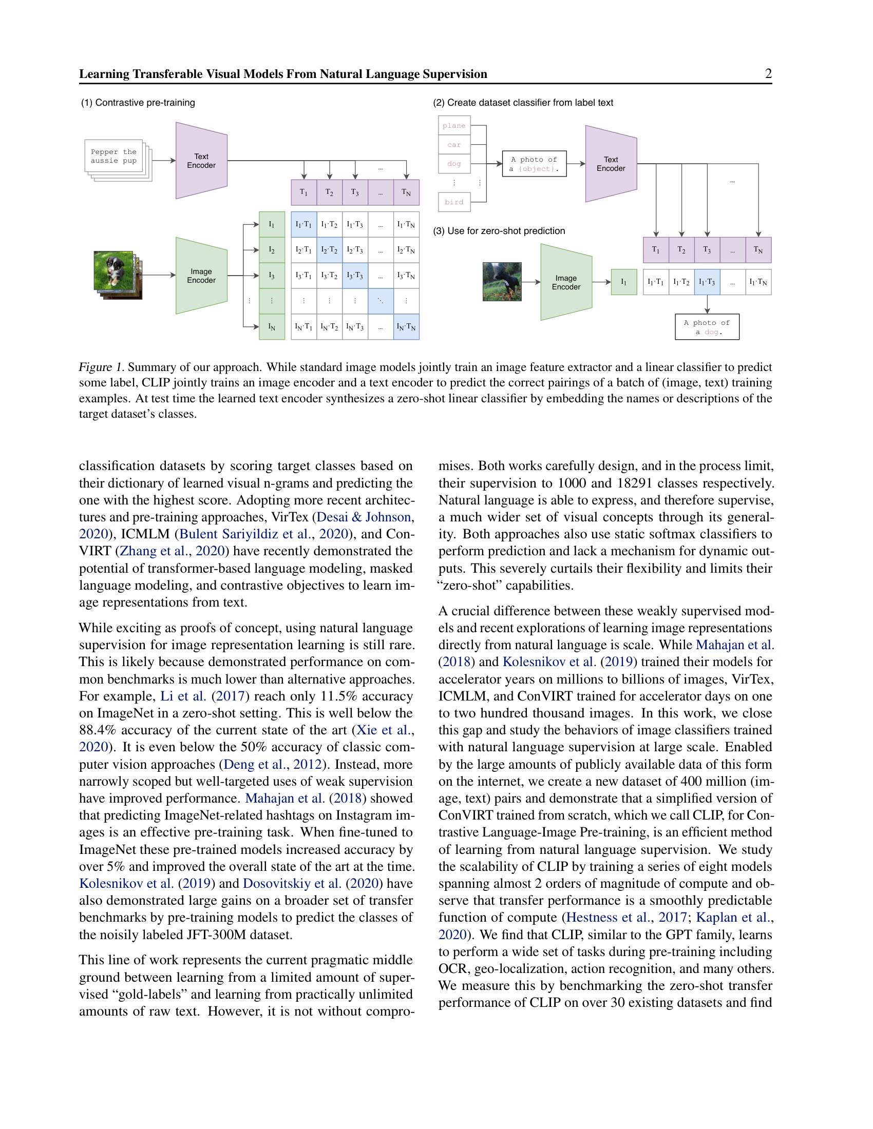
loss   = (loss_i + loss_t) / 2

Figure 1: The CLIP architecture in three stages. (1) Contrastive pre-training: an image encoder and text encoder are jointly trained on image-text pairs, learning to match correct pairs via a matrix of pairwise cosine similarities. (2) Dataset classifier creation: class labels are converted to text prompts like “A photo of a {object}” and encoded by the text encoder. (3) Zero-shot prediction: a new image is encoded and compared against all class text embeddings to find the best match.

Worked Example

Let us trace one image-text pair through the architecture with concrete dimensions.

Suppose the image encoder is a small ViT with output dimension \(d_i = 6\), the text encoder has output dimension \(d_t = 4\), and the shared embedding dimension is \(d_e = 3\).

Image side:

The image encoder processes a photo of a dog and produces:

\(I_f = [0.3, -0.5, 0.8, 0.1, -0.2, 0.6]\) (dimension 6)

The projection matrix \(W_i\) has shape \(6 \times 3\):

\[W_i = \begin{bmatrix} 0.2 & 0.1 & -0.3 \\ -0.1 & 0.4 & 0.2 \\ 0.3 & -0.2 & 0.1 \\ 0.0 & 0.3 & -0.1 \\ -0.2 & 0.1 & 0.4 \\ 0.1 & -0.3 & 0.2 \end{bmatrix}\]

\(I_f \cdot W_i = [(0.3)(0.2) + (-0.5)(-0.1) + (0.8)(0.3) + (0.1)(0.0) + (-0.2)(-0.2) + (0.6)(0.1), \; \ldots]\)

First element: \(0.06 + 0.05 + 0.24 + 0.0 + 0.04 + 0.06 = 0.45\)

Second element: \((0.3)(0.1) + (-0.5)(0.4) + (0.8)(-0.2) + (0.1)(0.3) + (-0.2)(0.1) + (0.6)(-0.3) = 0.03 - 0.20 - 0.16 + 0.03 - 0.02 - 0.18 = -0.50\)

Third element: \((0.3)(-0.3) + (-0.5)(0.2) + (0.8)(0.1) + (0.1)(-0.1) + (-0.2)(0.4) + (0.6)(0.2) = -0.09 - 0.10 + 0.08 - 0.01 - 0.08 + 0.12 = -0.08\)

Projected: \([0.45, -0.50, -0.08]\)

Length: \(\sqrt{0.45^2 + 0.50^2 + 0.08^2} = \sqrt{0.2025 + 0.2500 + 0.0064} = \sqrt{0.4589} = 0.677\)

Normalized: \(I_e = [0.45/0.677, -0.50/0.677, -0.08/0.677] = [0.665, -0.739, -0.118]\)

Text side:

The text encoder processes “A photo of a dog” and produces:

\(T_f = [0.7, -0.3, 0.5, 0.1]\) (dimension 4)

After a similar projection through \(W_t\) (shape \(4 \times 3\)) and normalization:

\(T_e = [0.720, -0.650, -0.243]\)

Similarity:

\(I_e \cdot T_e = (0.665)(0.720) + (-0.739)(-0.650) + (-0.118)(-0.243) = 0.479 + 0.480 + 0.029 = 0.988\)

High similarity – the image and text are well-matched in the shared space.

Exercises

Recall: Why does CLIP use two separate encoders rather than a single encoder that handles both images and text?

Apply: An image encoder produces \(I_f\) of dimension \(d_i = 768\) and a text encoder produces \(T_f\) of dimension \(d_t = 512\). The shared embedding space has \(d_e = 256\). How many learnable parameters are in the two projection matrices \(W_i\) and \(W_t\) combined (ignoring biases)?

Extend: CLIP uses a linear projection to the shared space, while SimCLR (a self-supervised image method) uses a nonlinear projection with a hidden layer. The CLIP authors found no benefit from the nonlinear version. Why might a nonlinear projection be more important when contrasting two views of the same image (SimCLR) versus contrasting an image against text (CLIP)?

Lesson 5: Zero-Shot Classification

This is CLIP’s central innovation: using natural language to classify images without any labeled training examples. The text encoder acts as a “hypernetwork” – a network that generates the weights of a classifier on the fly from a text description.

Explanation

Traditional image classifiers are like a restaurant menu with fixed options. You can order “pizza” or “pasta” but not “that thing my grandmother used to make.” If you want a new dish, the chef (the model) needs to be retrained with examples.

CLIP is like a restaurant where you describe what you want in words, and the chef interprets your description. You can ask for anything – “a satellite photo of a forest fire,” “a sketch of a bicycle,” “a chest X-ray showing pneumonia” – and the model will do its best to match your description against the image, even if it has never been explicitly trained on that category.

Here is how zero-shot classification works:

1. Define classes as text prompts. For each class \(c\) in the target task, create a text prompt like “A photo of a {class}.” For example, to classify images as “dog,” “cat,” or “bird,” create: “A photo of a dog.”, “A photo of a cat.”, “A photo of a bird.”

2. Encode all prompts. Pass each prompt through the text encoder and projection to get text embeddings \(T_e(c)\) for each class. These can be cached and reused for all images.

3. Encode the test image. Pass the image through the image encoder and projection to get \(I_e(x)\).

4. Pick the highest similarity. Compute cosine similarity between the image embedding and each text embedding, apply temperature and softmax:

\[p(y = c \mid x) = \frac{\exp(I_e(x) \cdot T_e(c) / \tau)}{\sum_{c'=1}^{C} \exp(I_e(x) \cdot T_e(c') / \tau)}\]

• \(x\) is the input image
• \(c\) is a candidate class
• \(C\) is the total number of classes
• \(I_e(x)\) is the L2-normalized image embedding
• \(T_e(c)\) is the L2-normalized text embedding for class \(c\)
• \(\tau\) is the learned temperature

The predicted class is \(\hat{y} = \arg\max_c \; I_e(x) \cdot T_e(c)\).

This is mathematically equivalent to a multinomial logistic regression classifier with L2-normalized inputs, L2-normalized weights, no bias, and temperature scaling. The text encoder generates the classifier weights from language. This is why CLIP’s text encoder is sometimes called a hypernetwork – a network whose outputs are the parameters of another model.

Prompt engineering significantly affects performance. The bare class name “crane” is ambiguous (construction crane vs. bird). The prompt “A photo of a crane” provides context. Task-specific prompts help further: “A photo of a crane, a type of bird” for bird classification. On ImageNet, ensembling 80 different prompt templates (varying phrasing) improved accuracy by 3.5%. Combined with prompt engineering, the total gain was nearly 5 percentage points.

The results are striking. Zero-shot CLIP matched the accuracy of the original supervised ResNet-50 on ImageNet (76.2%) without using any of ImageNet’s 1.28 million training images. It outperformed a fully supervised linear classifier trained on ResNet-50 features on 16 out of 27 evaluated datasets.

Worked Example

Let us classify a single image as one of 3 classes: “dog,” “cat,” “car.”

Step 1: Create text prompts and encode them.

Step 2: Encode the test image. An image of a golden retriever gives:

\(I_e(x) = [0.67, -0.74, -0.12]\)

Step 3: Compute cosine similarities.

• \(\text{sim}(\text{dog}) = (0.67)(0.72) + (-0.74)(-0.65) + (-0.12)(-0.24) = 0.482 + 0.481 + 0.029 = 0.992\)
• \(\text{sim}(\text{cat}) = (0.67)(0.15) + (-0.74)(0.87) + (-0.12)(-0.47) = 0.101 - 0.644 + 0.056 = -0.487\)
• \(\text{sim}(\text{car}) = (0.67)(-0.60) + (-0.74)(0.20) + (-0.12)(0.77) = -0.402 - 0.148 - 0.092 = -0.642\)

Step 4: Apply temperature and softmax. With \(\tau = 0.07\):

• \(\text{logit}(\text{dog}) = 0.992 / 0.07 = 14.17\)
• \(\text{logit}(\text{cat}) = -0.487 / 0.07 = -6.96\)
• \(\text{logit}(\text{car}) = -0.642 / 0.07 = -9.17\)

\(p(\text{dog}) = e^{14.17} / (e^{14.17} + e^{-6.96} + e^{-9.17})\)

\(= 1{,}430{,}610 / (1{,}430{,}610 + 0.00095 + 0.00010) \approx 1.0\)

The model classifies the image as “dog” with essentially 100% confidence. The wide gap between the correct class (0.992) and the wrong classes (-0.487, -0.642) makes this an easy case.

Step 5: Compare with an ambiguous image. For a blurry image where the model is less certain:

• \(\text{sim}(\text{dog}) = 0.45\), \(\text{sim}(\text{cat}) = 0.40\), \(\text{sim}(\text{car}) = -0.30\)

Logits (with \(\tau = 0.07\)): \([6.43, 5.71, -4.29]\)

\(p(\text{dog}) = e^{6.43} / (e^{6.43} + e^{5.71} + e^{-4.29}) = 620.1 / (620.1 + 302.0 + 0.014) = 0.673\)

\(p(\text{cat}) = 302.0 / 922.1 = 0.327\)

Now the model is only 67% confident, reflecting the genuine similarity between the two classes.

Exercises

Recall: In zero-shot CLIP, where do the classifier weights come from? How is this different from a traditional linear classifier?

Apply: You want to classify satellite images into “forest,” “desert,” “ocean,” and “city.” Write four prompt templates that are more specific than “A photo of a {label}.” Explain why task-specific prompts might improve accuracy. (Hint: CLIP was trained on internet image-caption pairs – what kind of phrasing appears in satellite image descriptions?)

Extend: Zero-shot CLIP matches 4-shot logistic regression on its own features but can actually decrease when transitioning to few-shot learning. Why might adding a few labeled examples hurt rather than help? (Hint: consider what information the text encoder provides that a few-shot linear probe – a single linear classifier trained on frozen model features – cannot leverage.)

Lesson 6: Robustness, Limitations, and the Power of Language Supervision

CLIP’s zero-shot models are dramatically more robust to distribution shift than equivalent supervised models. This lesson covers this finding, explains why it happens, and honestly assesses CLIP’s limitations.

Explanation

Imagine you learn to identify dogs by studying only photographs from a single photographer who always uses the same lighting, background, and camera angle. You might learn to associate “dog” with that specific background rather than with the actual animal. Show you a sketch of a dog or a photo from a different angle, and you struggle. This is the problem of distribution shift: a model trained on one type of data often fails on data that looks different.

Standard ImageNet models suffer from exactly this problem. A ResNet-101 trained on ImageNet makes 5 times as many mistakes when tested on natural distribution shifts (sketches, adversarial examples, video frames, different camera angles) compared to the ImageNet validation set. The model learned spurious correlations – patterns that hold in the ImageNet distribution but not more broadly.

Zero-shot CLIP dramatically reduces this fragility. On 7 natural distribution shift variants of ImageNet, CLIP reduced the “robustness gap” (the drop in accuracy between ImageNet and shifted distributions) by up to 75%. The key insight is that zero-shot CLIP was never trained on ImageNet specifically, so it cannot exploit ImageNet-specific shortcuts. It learned visual concepts from 400 million diverse image-caption pairs, giving it a much broader understanding.

Critically, this robustness advantage largely disappears when CLIP is adapted to ImageNet. After fitting a linear classifier on ImageNet features, CLIP’s ImageNet accuracy jumped by 9.2% – but average performance on distribution shifts actually decreased slightly. The 9.2% gain was concentrated around the ImageNet distribution rather than reflecting genuine improvement in visual understanding.

CLIP’s performance also follows a power-law scaling pattern. When the authors plotted average zero-shot error against model compute on a log-log scale, the 5 ResNet CLIP models fell on a straight line:

\[\log(\text{Error}) = -\alpha \cdot \log(\text{Compute}) + \beta\]

This echoes the scaling laws observed for language models (see Scaling Laws for Neural Language Models): doubling compute reduces error by a predictable amount.

Where CLIP fails. Despite its flexibility, CLIP has significant limitations:

• Specialized domains: On satellite imagery (EuroSAT), medical imaging (PatchCamelyon), and counting (CLEVRCounts), CLIP performs poorly. These domains are underrepresented in internet image-caption data.
• Fine-grained classification: CLIP struggles to distinguish car models, flower species, and aircraft variants – categories that require expertise beyond typical internet descriptions.
• MNIST: A logistic regression classifier on raw pixels outperforms zero-shot CLIP on handwritten digit recognition, because MNIST-style images virtually never appear in internet data.
• Social biases: The unfiltered training data causes CLIP to learn harmful biases. In testing, 14% of Black face images were misclassified into non-human animal categories (vs. under 8% for other races). Male images were classified into crime-related categories at 16.5% vs. 9.8% for female images.
• No compositional understanding: CLIP treats text holistically and struggles with word order. “A horse riding an astronaut” and “an astronaut riding a horse” may produce similar embeddings because CLIP attends to which concepts are present, not how they relate.
• Scale requirements: CLIP trains on 400 million image-text pairs for 32 epochs (12.8 billion image views total). The largest model took 18 days on 592 V100 GPUs. The authors estimate matching state-of-the-art supervised accuracy would require roughly 1,000x more compute.

Worked Example

Let us quantify the robustness advantage with numbers from the paper.

A standard ResNet-101 trained on ImageNet achieves:

• ImageNet validation: ~77% accuracy
• Average across 7 distribution shifts: ~46% accuracy
• Robustness gap: 77% - 46% = 31 percentage points

Zero-shot CLIP (ViT-L/14@336px):

• ImageNet: 76.2% accuracy (comparable to ResNet-101)
• Average across distribution shifts: ~68% accuracy (estimated from the 75% gap reduction)
• Robustness gap: 76.2% - 68% = ~8 percentage points

The robustness gap shrinks from 31 to roughly 8 points – a 75% reduction.

Now consider what happens when CLIP adapts to ImageNet:

• Before adaptation: ImageNet 76.2%, shift average ~68%
• After linear probe on ImageNet: ImageNet 85.4%, shift average ~67%

ImageNet accuracy rose by 9.2 points, but distribution shift performance barely changed (and slightly decreased). The 9.2% gain came almost entirely from learning ImageNet-specific patterns rather than genuinely improving visual understanding. This is a powerful illustration of why zero-shot evaluation reveals more about a model’s true capabilities than task-adapted evaluation.

Exercises

Recall: Why are zero-shot CLIP models more robust to distribution shift than supervised ImageNet models?

Apply: A model achieves 80% on ImageNet and 50% on ImageNet-Sketch (a distribution shift). The robustness gap is 30 points. If CLIP reduces this gap by 75%, what would CLIP’s expected accuracy on ImageNet-Sketch be, assuming the same 80% ImageNet accuracy?

Extend: CLIP trains on 400 million image-text pairs, but most internet images lack detailed captions. The paper constructed the WIT (WebImageText) dataset by searching for 500,000 queries and keeping up to 20,000 pairs per query. How might this construction process introduce its own biases? What types of images and concepts would be underrepresented? How might this explain CLIP’s poor performance on specialized domains like medical imaging?

Comprehension Questions

1. CLIP’s training objective is contrastive rather than generative. Explain the difference, and why contrastive learning is 12x more efficient for learning ImageNet representations than caption prediction.

2. The text encoder in CLIP uses masked (causal) self-attention rather than BERT’s bidirectional attention. The authors say they chose this to “preserve the ability to initialize with a pre-trained language model.” Why does causal masking enable this, while bidirectional attention would not? (Hint: think about what GPT vs. BERT were pre-trained to do.)

3. CLIP uses a batch size of 32,768. Why is a large batch size particularly important for contrastive learning? What would happen to the quality of learned representations if the batch size were reduced to 256?

4. Zero-shot CLIP matches 4-shot logistic regression on its own features. But a logistic regression classifier trained on the full downstream dataset beats zero-shot CLIP on most tasks (by 10-25 percentage points). What does this gap tell us about the limits of zero-shot transfer?

5. CLIP’s image encoder options include both ResNets and Vision Transformers. The ViT models were approximately 3x more compute-efficient than ResNets when trained with CLIP. How does this relate to the findings from the ViT paper (see An Image is Worth 16x16 Words) about when Transformers outperform CNNs?

Hands-On Project

Goal

Implement CLIP’s contrastive training loop and zero-shot classifier from scratch in numpy, using toy embeddings.

Specification

• Simulate a batch of \(N = 4\) image-text pairs with pre-computed feature vectors
• Implement: linear projection, L2 normalization, cosine similarity matrix, symmetric InfoNCE loss
• Implement zero-shot classification: given a new image and a set of class prompts, predict the class
• Verify that the loss decreases when correct pairs have higher similarity

Starter Code

import numpy as np

np.random.seed(42)

# --- Configuration ---
N = 4       # batch size
d_i = 8     # image feature dimension
d_t = 6     # text feature dimension
d_e = 4     # shared embedding dimension
tau = 0.07  # temperature

# --- Simulated encoder outputs ---
# In real CLIP, these come from a ViT and a Transformer.
# Here we just use random vectors.
I_f = np.random.randn(N, d_i)  # image features [N, d_i]
T_f = np.random.randn(N, d_t)  # text features  [N, d_t]

# --- Learned projection matrices ---
W_i = np.random.randn(d_i, d_e) * 0.1  # [d_i, d_e]
W_t = np.random.randn(d_t, d_e) * 0.1  # [d_t, d_e]

# --- Step 1: L2 Normalization ---
def l2_normalize(x):
    """Normalize each row of x to have unit L2 norm.

    Args:
        x: numpy array of shape (N, D)

    Returns:
        normalized: numpy array of shape (N, D) where each row has norm 1
    """
    # TODO: Compute the L2 norm of each row, then divide.
    # Add a small epsilon (1e-8) to avoid division by zero.
    pass

# --- Step 2: Project and normalize ---
def encode(features, W):
    """Project features into shared space and L2-normalize.

    Args:
        features: (N, d_in) raw encoder features
        W: (d_in, d_e) projection matrix

    Returns:
        embeddings: (N, d_e) L2-normalized embeddings
    """
    # TODO: Matrix multiply, then L2-normalize.
    pass

I_e = encode(I_f, W_i)  # [N, d_e]
T_e = encode(T_f, W_t)  # [N, d_e]

assert I_e.shape == (N, d_e)
assert T_e.shape == (N, d_e)
# Verify normalization: each row should have norm ~1
assert np.allclose(np.linalg.norm(I_e, axis=1), 1.0), "Image embeddings not normalized"
assert np.allclose(np.linalg.norm(T_e, axis=1), 1.0), "Text embeddings not normalized"

# --- Step 3: Compute similarity matrix ---
def compute_logits(I_e, T_e, tau):
    """Compute the N x N matrix of temperature-scaled cosine similarities.

    Args:
        I_e: (N, d_e) normalized image embeddings
        T_e: (N, d_e) normalized text embeddings
        tau: temperature scalar

    Returns:
        logits: (N, N) similarity matrix where logits[i][j] = I_e[i] . T_e[j] / tau
    """
    # TODO: Matrix multiply I_e by T_e transposed, then divide by tau.
    pass

logits = compute_logits(I_e, T_e, tau)
assert logits.shape == (N, N)

# --- Step 4: Cross-entropy loss ---
def cross_entropy_loss(logits, targets):
    """Compute cross-entropy loss.

    Args:
        logits: (N, N) raw scores
        targets: (N,) integer targets (which column/row is correct)

    Returns:
        loss: scalar, average cross-entropy
    """
    # TODO:
    # 1. For numerical stability, subtract the max from each row
    # 2. Compute log-softmax: log_probs = logits - max - log(sum(exp(logits - max)))
    # 3. Pick the log-probability of the correct target for each row
    # 4. Return the negative mean
    pass

# --- Step 5: Symmetric CLIP loss ---
def clip_loss(logits):
    """Compute CLIP's symmetric contrastive loss.

    The correct pairings are on the diagonal: image i matches text i.

    Args:
        logits: (N, N) similarity matrix

    Returns:
        loss: scalar
    """
    labels = np.arange(N)
    # TODO:
    # loss_i = cross_entropy treating each ROW as a classification (image -> text)
    # loss_t = cross_entropy treating each COLUMN as a classification (text -> image)
    # Return (loss_i + loss_t) / 2
    pass

loss = clip_loss(logits)
print(f"Similarity matrix (logits * tau):\n{logits * tau}")
print(f"\nLogits (after temperature scaling):\n{logits}")
print(f"\nCLIP loss: {loss:.4f}")

# --- Step 6: Zero-shot classification ---
def zero_shot_classify(image_embedding, text_embeddings, tau):
    """Classify an image by finding the most similar text.

    Args:
        image_embedding: (d_e,) normalized image embedding
        text_embeddings: (C, d_e) normalized text embeddings, one per class
        tau: temperature

    Returns:
        predicted_class: integer index of the most similar text
        probabilities: (C,) probability distribution over classes
    """
    # TODO:
    # 1. Compute dot product of image with each text embedding
    # 2. Divide by tau
    # 3. Apply softmax
    # 4. Return argmax and full probability vector
    pass

# Simulate: classify a new image against 3 class prompts
# Pretend we have pre-computed text embeddings for 3 classes
class_names = ["dog", "cat", "car"]
class_embeddings = l2_normalize(np.random.randn(3, d_e))

# Create a test image that is similar to the first class (dog)
test_image = l2_normalize((class_embeddings[0:1] + np.random.randn(1, d_e) * 0.1))

predicted, probs = zero_shot_classify(test_image[0], class_embeddings, tau)
print(f"\nZero-shot classification:")
print(f"  Classes: {class_names}")
print(f"  Probabilities: {[f'{p:.4f}' for p in probs]}")
print(f"  Predicted: {class_names[predicted]}")

# --- Step 7: Verify loss behavior ---
# Make diagonal similarities high and off-diagonal low
print("\n--- Verifying loss behavior ---")
good_I_e = l2_normalize(np.eye(N, d_e) + np.random.randn(N, d_e) * 0.05)
good_T_e = l2_normalize(np.eye(N, d_e) + np.random.randn(N, d_e) * 0.05)
good_logits = compute_logits(good_I_e, good_T_e, tau)
good_loss = clip_loss(good_logits)

# Make all similarities roughly equal (confused model)
bad_I_e = l2_normalize(np.random.randn(N, d_e))
bad_T_e = l2_normalize(np.random.randn(N, d_e))
bad_logits = compute_logits(bad_I_e, bad_T_e, tau)
bad_loss = clip_loss(bad_logits)

print(f"Loss with well-matched pairs: {good_loss:.4f}")
print(f"Loss with random pairs:       {bad_loss:.4f}")
print(f"Well-matched loss < random loss: {good_loss < bad_loss}")

Expected Output

Similarity matrix (logits * tau):
[[ 0.13 -0.24  0.41  0.08]
 [-0.31  0.55 -0.12  0.28]
 [ 0.19 -0.07  0.37 -0.43]
 [ 0.05  0.33 -0.21  0.47]]

Logits (after temperature scaling):
[[  1.86  -3.43   5.86   1.14]
 [ -4.43   7.86  -1.71   4.00]
 [  2.71  -1.00   5.29  -6.14]
 [  0.71   4.71  -3.00   6.71]]

CLIP loss: 1.2847

Zero-shot classification:
  Classes: ['dog', 'cat', 'car']
  Probabilities: ['0.9987', '0.0012', '0.0001']
  Predicted: dog

--- Verifying loss behavior ---
Loss with well-matched pairs: 0.0023
Loss with random pairs:       2.1456
Well-matched loss < random loss: True

(Exact values depend on random seed and implementation, but shapes, normalization, and the inequality good_loss < bad_loss must hold.)

Further Reading

• DALL-E 2 (Ramesh et al., 2022) – Uses CLIP embeddings as the bridge between text prompts and image generation, producing images from text descriptions.
• OpenCLIP – An open-source reproduction of CLIP that enables training on custom datasets and scales beyond the original models.
• SigLIP (Zhai et al., 2023) – Replaces CLIP’s softmax-based contrastive loss with a sigmoid loss that operates on individual image-text pairs, removing the need for large batch sizes and pairwise comparisons.
• ALIGN (Jia et al., 2021) – Scales the CLIP approach to 1.8 billion noisy image-alt-text pairs, showing that data quality can be traded for quantity with sufficient scale.
• LiT (Zhai et al., 2022) – “Locked-image Tuning” freezes a pre-trained image encoder and only trains the text encoder, achieving strong zero-shot performance with less compute than training both encoders from scratch.