By the end of this course, you will be able to:
Why would you deliberately ruin an image by adding static? Because if you can learn to undo that damage – to look at a noisy image and predict what the clean version looked like – you have learned something deep about the structure of images. And if you can do that starting from pure static, you can create images that never existed. The entire diffusion framework rests on one specific type of noise: the Gaussian distribution.
A Gaussian distribution (also called a normal distribution) is a bell-shaped probability distribution defined by two parameters: a mean \(\mu\) (the center) and a variance \(\sigma^2\) (how spread out it is). We write this as \(\mathcal{N}(\mu, \sigma^2)\). When \(\mu = 0\) and \(\sigma^2 = 1\), we call it the standard normal distribution.
For images, noise means adding a random value to each pixel independently. If we have a grayscale pixel with value 0.5 and we add noise sampled from \(\mathcal{N}(0, 0.01)\), the result is a new pixel value centered at 0.5 with a small random perturbation. With variance 0.01, the noise is barely visible. With variance 1.0, the noise overwhelms the signal.
Gaussians have a crucial property that makes the entire diffusion framework work: the sum of two independent Gaussian random variables is itself Gaussian. If \(X \sim \mathcal{N}(\mu_1, \sigma_1^2)\) and \(Y \sim \mathcal{N}(\mu_2, \sigma_2^2)\) are independent, then:
\[X + Y \sim \mathcal{N}(\mu_1 + \mu_2,\; \sigma_1^2 + \sigma_2^2)\]
This means that if you add noise to a signal, then add more noise, the result is the same as if you had added a single larger dose of noise. This composability is what enables the closed-form shortcut we will derive in Lesson 3.
For images with multiple pixels, we use a multivariate Gaussian \(\mathcal{N}(\mu, \sigma^2 I)\), where \(I\) is the identity matrix (meaning noise is added independently to each pixel with the same variance). The notation \(\epsilon \sim \mathcal{N}(0, I)\) means we sample a noise vector where every element is drawn independently from a standard normal.
Let a tiny 1x2 “image” have pixel values \(x = [0.8, -0.3]\). We add Gaussian noise with variance \(\sigma^2 = 0.1\):
The noisy image is a sample from \(\mathcal{N}(x, 0.1 \cdot I) = \mathcal{N}([0.8, -0.3], 0.1 \cdot I)\).
Now add a second round of noise with variance \(0.2\). Sample \(\epsilon_2 = [-0.55, 0.38]\), scale by \(\sqrt{0.2} \approx 0.447\): \([-0.246, 0.170]\). Result: \([0.933 - 0.246, -0.524 + 0.170] = [0.687, -0.354]\).
By the Gaussian addition property, this two-step result has the same distribution as adding noise with total variance \(0.1 + 0.2 = 0.3\) in a single step. The intermediate step does not matter – only the total accumulated noise.
Recall: What property of Gaussian distributions makes it possible to skip intermediate noise-addition steps and jump directly to any noise level?
Apply: A pixel has value 0.6. You add noise \(\epsilon_1 \sim \mathcal{N}(0, 0.05)\), then add noise \(\epsilon_2 \sim \mathcal{N}(0, 0.15)\). What single Gaussian distribution describes the result? Write it as \(\mathcal{N}(\mu, \sigma^2)\).
Extend: If you keep adding small amounts of noise indefinitely, what distribution does the image converge to? Why does the original image content get destroyed?
Imagine you have a photograph and you make 1000 photocopies in sequence, where each copy introduces a tiny amount of static. By copy 1000, the image is pure static. The forward process in DDPM formalizes this as a Markov chain – a sequence where each step depends only on the previous one.
The forward process takes a clean image \(x_0\) from the training set and produces a sequence of increasingly noisy versions \(x_1, x_2, \ldots, x_T\) over \(T = 1000\) steps. At each step \(t\), the transition is:
\[q(x_t | x_{t-1}) = \mathcal{N}(x_t;\, \sqrt{1-\beta_t}\, x_{t-1},\, \beta_t I)\]
In plain language: take the previous image, shrink it slightly (multiply by \(\sqrt{1-\beta_t}\)), and add Gaussian noise with variance \(\beta_t\). The shrinking is important – without it, the total variance would grow without bound. By shrinking the signal slightly at each step, the process keeps the total variance controlled and converges to a standard normal distribution \(\mathcal{N}(0, I)\).
The variance schedule \(\beta_1, \ldots, \beta_T\) controls how quickly the image is destroyed. The paper uses a linear schedule from \(\beta_1 = 10^{-4}\) to \(\beta_T = 0.02\). Early steps add almost no noise (the image looks nearly unchanged). Later steps add more. By step 1000, the result is indistinguishable from pure random noise.
The full forward process is the product of all individual transitions:
\[q(x_{1:T} | x_0) = \prod_{t=1}^T q(x_t | x_{t-1})\]
This is a Markov chain because each step depends only on the immediately previous state, not on any earlier history.
Let a 1-pixel “image” have value \(x_0 = 0.9\). Use \(\beta_1 = 0.0001\) and \(\beta_2 = 0.0002\).
Step 1 (\(t=1\)):
The image barely changed. With \(\beta_1 = 0.0001\), the noise standard deviation is only 0.01.
Step 2 (\(t=2\)):
After two steps, \(x_0 = 0.9\) has become \(x_2 = 0.890\). Still recognizable. After 1000 steps with increasing \(\beta_t\), the signal is completely buried.
Recall: Why does the forward process multiply \(x_{t-1}\) by \(\sqrt{1-\beta_t}\) before adding noise? What would happen without this scaling?
Apply: Given \(x_0 = 0.5\), \(\beta_1 = 0.001\), and a noise sample \(\epsilon = -0.8\), compute \(x_1\).
Extend: The paper uses \(T = 1000\) steps with tiny \(\beta_t\) values. Would \(T = 10\) steps with larger \(\beta_t\) achieve the same result? What might go wrong?
Computing \(x_{500}\) by running 500 sequential noise-addition steps would be absurdly wasteful during training. A cornerstone of the DDPM approach is that Gaussians compose: you can jump from \(x_0\) directly to \(x_t\) for any \(t\) in a single computation. This shortcut is what makes training practical.
We define two useful quantities:
\[\alpha_t = 1 - \beta_t \qquad \bar{\alpha}_t = \prod_{s=1}^{t} \alpha_s\]
Because each forward step is Gaussian, and Gaussians compose (as we learned in Lesson 1), the distribution of \(x_t\) given \(x_0\) has a closed form:
\[q(x_t | x_0) = \mathcal{N}(x_t;\, \sqrt{\bar{\alpha}_t}\, x_0,\, (1 - \bar{\alpha}_t) I)\]
This means we can sample \(x_t\) directly:
\[x_t = \sqrt{\bar{\alpha}_t}\, x_0 + \sqrt{1 - \bar{\alpha}_t}\, \epsilon, \quad \text{where } \epsilon \sim \mathcal{N}(0, I)\]
Think of this as a weighted mix between the clean image (\(x_0\)) and pure noise (\(\epsilon\)). Early in the process (\(t\) small), \(\bar{\alpha}_t \approx 1\), so the clean image dominates. Late in the process (\(t\) large), \(\bar{\alpha}_t \approx 0\), so noise dominates.
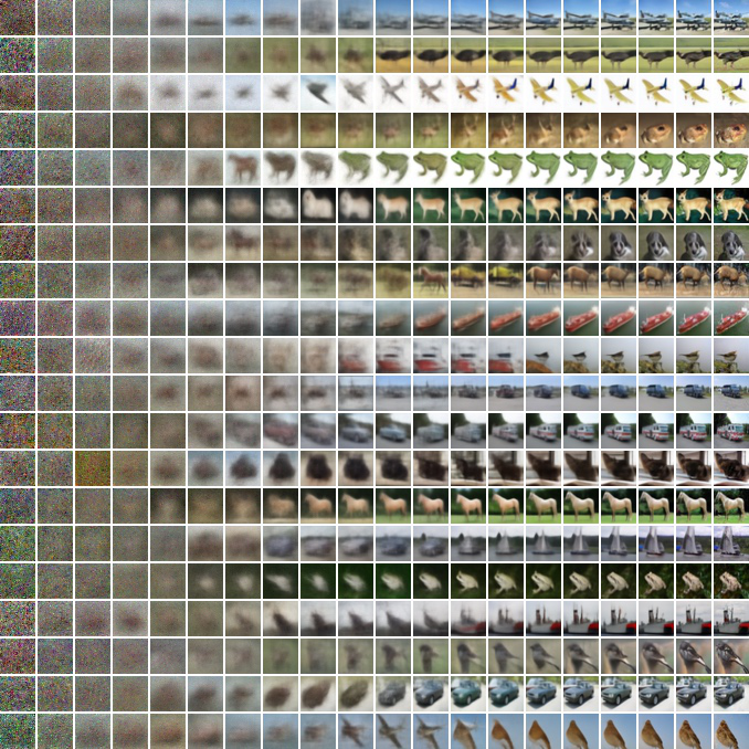
Progressive denoising on CIFAR10 (a dataset of 32x32 color images across 10 categories like cars, birds, and horses): the model’s estimated clean image \(\hat{x}_0\) at various points during the 1000-step reverse process (left to right). Large-scale structure like color and shape emerges first; fine details appear last. Each row is a different sample being generated from pure noise.
Let \(x_0 = 0.9\) (a 1-pixel image). Use a 3-step schedule with \(\beta_1 = 0.1\), \(\beta_2 = 0.2\), \(\beta_3 = 0.3\).
First, compute the \(\alpha\) and \(\bar{\alpha}\) values:
| \(t\) | \(\beta_t\) | \(\alpha_t = 1 - \beta_t\) | \(\bar{\alpha}_t = \prod_{s=1}^{t}\alpha_s\) |
|---|---|---|---|
| 1 | 0.1 | 0.9 | 0.9 |
| 2 | 0.2 | 0.8 | \(0.9 \times 0.8 = 0.72\) |
| 3 | 0.3 | 0.7 | \(0.72 \times 0.7 = 0.504\) |
Now jump directly to \(t = 3\). Suppose \(\epsilon = 0.65\):
\[x_3 = \sqrt{0.504} \times 0.9 + \sqrt{1 - 0.504} \times 0.65 = 0.710 \times 0.9 + 0.704 \times 0.65 = 0.639 + 0.458 = 1.097\]
At \(t=3\), roughly half the variance comes from the original signal and half from noise. At \(t = 1000\) with the paper’s schedule, \(\bar{\alpha}_{1000} \approx 0.00006\), meaning 99.99% of the variance is noise – the original image is effectively erased.
This shortcut is critical for training: to compute the loss at a random timestep \(t\), we generate \(x_t\) in \(O(1)\) time rather than running \(t\) sequential steps.
Recall: What does \(\bar{\alpha}_t\) represent intuitively? What happens to its value as \(t\) increases from 1 to \(T\)?
Apply: Given \(\beta_1 = 0.01\), \(\beta_2 = 0.02\), \(\beta_3 = 0.03\), compute \(\bar{\alpha}_3\). Then compute \(x_3\) for \(x_0 = 0.7\) and \(\epsilon = -0.5\).
Extend: The paper chooses \(\beta_t\) to increase linearly from \(10^{-4}\) to \(0.02\). How would the behavior change if \(\beta_t\) were constant at \(0.01\) for all 1000 steps? Would \(\bar{\alpha}_{1000}\) be larger or smaller than with the linear schedule?
The forward process is easy: just add noise. The hard part is going backward. Given a noisy image \(x_t\), can we recover the slightly less noisy \(x_{t-1}\)? If we can, we chain 1000 such steps starting from pure noise and get a clean image. This is the generative direction – and the reason diffusion models exist.
The reverse process learns to undo the forward process one step at a time. Each reverse step is modeled as a Gaussian:
\[p_\theta(x_{t-1} | x_t) = \mathcal{N}(x_{t-1};\, \mu_\theta(x_t, t),\, \sigma_t^2 I)\]
The neural network takes two inputs: the current noisy image \(x_t\) and the timestep \(t\) (an integer telling the network how noisy the input is). It outputs a prediction that is used to compute \(\mu_\theta\).
Why is a Gaussian the right choice for the reverse step? When the forward steps are small (small \(\beta_t\)), statistical theory guarantees that the true reverse transition is also approximately Gaussian. Since this paper uses 1000 tiny steps, the Gaussian assumption is well justified.
Now, here is a key insight. During training, we know the original image \(x_0\). If we condition the forward process posterior on \(x_0\), we get a tractable (computationally feasible to calculate in closed form) target distribution:
\[q(x_{t-1} | x_t, x_0) = \mathcal{N}(x_{t-1};\, \tilde{\mu}_t(x_t, x_0),\, \tilde{\beta}_t I)\]
where:
\[\tilde{\mu}_t(x_t, x_0) = \frac{\sqrt{\bar{\alpha}_{t-1}}\,\beta_t}{1-\bar{\alpha}_t}\,x_0 + \frac{\sqrt{\alpha_t}\,(1- \bar{\alpha}_{t-1})}{1-\bar{\alpha}_t}\, x_t\]
\[\tilde{\beta}_t = \frac{1-\bar{\alpha}_{t-1}}{1-\bar{\alpha}_t}\,\beta_t\]
In plain language: if we know both the noisy image \(x_t\) and the original \(x_0\), we can compute exactly where \(x_{t-1}\) should land. The posterior mean is a blend of the original image (pulling toward the truth) and the current noisy image (staying close to where we are). Training the model means making \(\mu_\theta(x_t, t)\) match \(\tilde{\mu}_t(x_t, x_0)\) as closely as possible.
Let \(x_0 = 0.9\), \(t = 2\), and use \(\beta_1 = 0.1\), \(\beta_2 = 0.2\). We computed \(\alpha_1 = 0.9\), \(\alpha_2 = 0.8\), \(\bar{\alpha}_1 = 0.9\), \(\bar{\alpha}_2 = 0.72\).
Suppose the noisy image at step 2 is \(x_2 = 1.1\) (we know this because we ran the forward process).
Compute the posterior mean \(\tilde{\mu}_2(x_2, x_0)\):
\[\tilde{\mu}_2 = \frac{\sqrt{0.9} \times 0.2}{1 - 0.72} \times 0.9 + \frac{\sqrt{0.8} \times (1 - 0.9)}{1 - 0.72} \times 1.1\]
\[= \frac{0.949 \times 0.2}{0.28} \times 0.9 + \frac{0.894 \times 0.1}{0.28} \times 1.1\]
\[= \frac{0.1897}{0.28} \times 0.9 + \frac{0.0894}{0.28} \times 1.1 = 0.678 \times 0.9 + 0.319 \times 1.1\]
\[= 0.610 + 0.351 = 0.961\]
The posterior variance: \(\tilde{\beta}_2 = \frac{1 - 0.9}{1 - 0.72} \times 0.2 = \frac{0.1}{0.28} \times 0.2 = 0.0714\).
So \(q(x_1 | x_2, x_0) = \mathcal{N}(0.961, 0.0714)\). The reverse step lands between the original value (0.9) and the noisy value (1.1), closer to the original – which is exactly what denoising should do.
Recall: Why can we compute the exact posterior \(q(x_{t-1} | x_t, x_0)\) during training but not during generation?
Apply: Given \(x_0 = 0.5\), \(x_2 = 0.7\), \(\bar{\alpha}_1 = 0.95\), \(\bar{\alpha}_2 = 0.85\), \(\alpha_2 = 0.85/0.95 \approx 0.895\), and \(\beta_2 = 1 - 0.895 = 0.105\), compute \(\tilde{\mu}_2\) and \(\tilde{\beta}_2\).
Extend: The posterior mean \(\tilde{\mu}_t\) is a weighted sum of \(x_0\) and \(x_t\). At early timesteps (\(t\) small, little noise), which term dominates? At late timesteps (\(t\) large, lots of noise)? Why does this make intuitive sense?
We now have a forward process that destroys data and a reverse process that tries to reconstruct it. How do we train the reverse process? The answer comes from variational inference – the same framework used in VAEs (see Auto-Encoding Variational Bayes course). We optimize a bound on the negative log-likelihood that decomposes into manageable per-timestep terms.
The goal of a generative model is to maximize the likelihood \(p_\theta(x_0)\) – the probability that the model assigns to real training images. Since computing this exactly is intractable (it requires integrating over all possible noise trajectories), we optimize a variational bound:
\[L = \mathbb{E}_q \bigg[ \underbrace{D_\text{KL}(q(x_T|x_0) \| p(x_T))}_{L_T} + \sum_{t > 1} \underbrace{D_\text{KL}(q(x_{t-1}|x_t,x_0) \| p_\theta(x_{t-1}|x_t))}_{L_{t-1}} \underbrace{- \log p_\theta(x_0|x_1)}_{L_0} \bigg]\]
This has three types of terms:
\(L_T\): measures how close the final noisy distribution \(q(x_T|x_0)\) is to the prior \(p(x_T) = \mathcal{N}(0, I)\). Since the forward process is fixed and \(T=1000\), this term is nearly zero and has no learnable parameters.
\(L_{t-1}\) for \(1 < t \leq T\): measures how close the learned reverse step \(p_\theta(x_{t-1}|x_t)\) is to the true posterior \(q(x_{t-1}|x_t,x_0)\). Each of these is a KL divergence between two Gaussians, which has a closed form.
\(L_0\): the reconstruction term, measuring how well the model recovers the final clean image from \(x_1\).
The KL divergence between two Gaussians \(\mathcal{N}(\mu_1, \sigma_1^2)\) and \(\mathcal{N}(\mu_2, \sigma_2^2)\) is:
\[D_\text{KL} = \log\frac{\sigma_2}{\sigma_1} + \frac{\sigma_1^2 + (\mu_1 - \mu_2)^2}{2\sigma_2^2} - \frac{1}{2}\]
When \(\sigma_1 = \sigma_2\) (same variance, which holds here because the paper fixes \(\sigma_t\)), this simplifies to:
\[D_\text{KL} = \frac{1}{2\sigma_t^2} \|\tilde{\mu}_t(x_t, x_0) - \mu_\theta(x_t, t)\|^2\]
This is just the squared distance between the true posterior mean and the model’s predicted mean, scaled by the variance. Training reduces to making \(\mu_\theta\) match \(\tilde{\mu}_t\) at every timestep.
Consider a single timestep \(t = 5\) for a 1-pixel image. Suppose \(\sigma_5^2 = 0.008\) (the fixed reverse variance), \(\tilde{\mu}_5 = 0.72\) (the true posterior mean), and \(\mu_\theta = 0.68\) (the model’s prediction).
The \(L_4\) term for this training example is:
\[L_4 = \frac{1}{2 \times 0.008} |0.72 - 0.68|^2 = \frac{1}{0.016} \times 0.0016 = 0.1\]
If the model had predicted \(\mu_\theta = 0.71\) (closer to truth):
\[L_4 = \frac{1}{0.016} \times |0.72 - 0.71|^2 = 62.5 \times 0.0001 = 0.00625\]
The loss dropped from 0.1 to 0.00625 – a 16x improvement from getting 0.03 closer to the true mean. This shows how the quadratic penalty amplifies even small errors.
Recall: What are the three types of terms in the variational bound \(L\)? Which one has no learnable parameters?
Apply: Given \(\sigma_t^2 = 0.01\), \(\tilde{\mu}_t = 0.55\), and \(\mu_\theta = 0.60\), compute the KL term \(L_{t-1}\) for this single timestep.
Extend: The variational bound has \(T - 1\) KL terms (one per timestep). If all terms were weighted equally, would the model spend equal effort on easy denoising (small \(t\), barely noisy images) and hard denoising (large \(t\), very noisy images)? What happens to the weighting factor \(\frac{1}{2\sigma_t^2}\) as \(t\) varies?
We know the model needs to predict the posterior mean \(\tilde{\mu}_t\). But what should the neural network actually output? It could predict the clean image \(x_0\), the mean \(\tilde{\mu}_t\) directly, or something else entirely. The paper’s key discovery is that predicting the noise \(\epsilon\) that was added works dramatically better than the alternatives. This is the central technical insight of DDPM.
Recall from Lesson 3 that we can write \(x_t\) as a mix of signal and noise:
\[x_t = \sqrt{\bar{\alpha}_t}\, x_0 + \sqrt{1 - \bar{\alpha}_t}\, \epsilon\]
This means we can express \(x_0\) in terms of \(x_t\) and \(\epsilon\):
\[x_0 = \frac{1}{\sqrt{\bar{\alpha}_t}} (x_t - \sqrt{1 - \bar{\alpha}_t}\, \epsilon)\]
If we substitute this into the posterior mean formula from Lesson 4, after some algebra we get:
\[\tilde{\mu}_t = \frac{1}{\sqrt{\alpha_t}} \left( x_t - \frac{\beta_t}{\sqrt{1 - \bar{\alpha}_t}}\, \epsilon \right)\]
This is a remarkable simplification. The posterior mean depends on \(x_t\) (which we have) and \(\epsilon\) (the noise that was added, which we do not know at generation time). So the authors propose: let the neural network predict \(\epsilon\). Define \(\epsilon_\theta(x_t, t)\) as the network’s noise prediction, and parameterize:
\[\mu_\theta(x_t, t) = \frac{1}{\sqrt{\alpha_t}} \left( x_t - \frac{\beta_t}{\sqrt{1 - \bar{\alpha}_t}}\, \epsilon_\theta(x_t, t) \right)\]
To sample \(x_{t-1}\) from \(p_\theta(x_{t-1}|x_t)\), we compute:
\[x_{t-1} = \frac{1}{\sqrt{\alpha_t}}\left( x_t - \frac{1 - \alpha_t}{\sqrt{1 - \bar{\alpha}_t}}\, \epsilon_\theta(x_t, t) \right) + \sigma_t z\]
where \(z \sim \mathcal{N}(0, I)\) if \(t > 1\), and \(z = 0\) if \(t = 1\) (no noise at the final step).
Why does noise prediction work better than directly predicting \(x_0\) or \(\tilde{\mu}_t\)? The paper shows that predicting \(\epsilon\) is mathematically equivalent to estimating the score function \(\nabla_x \log p(x)\) – the gradient of the log probability density of the noisy data. This connects DDPM to a separate line of research called denoising score matching. The score function points “uphill” toward higher probability regions, so a network that estimates it well is learning the structure of the data distribution at every noise level.
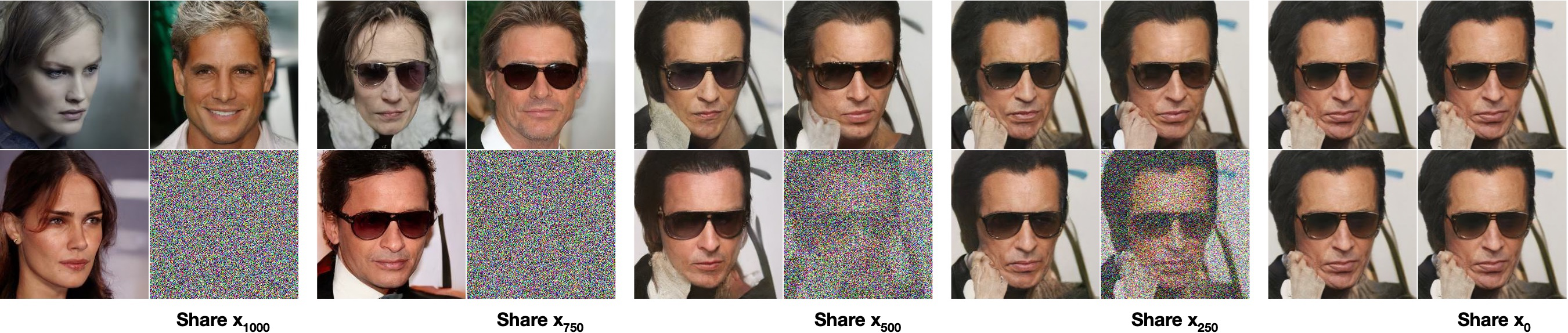
Samples generated from the same intermediate noisy image \(x_t\) at different noise levels. At \(t=1000\) (left), the shared latent is nearly pure noise, so samples differ completely. At \(t=250\) (right), most structure is preserved and samples differ only in fine details. This demonstrates the coarse-to-fine generation process.
Let \(x_0 = 0.9\), and suppose at \(t = 2\) with \(\alpha_2 = 0.8\), \(\bar{\alpha}_2 = 0.72\), \(\beta_2 = 0.2\), the noise was \(\epsilon = 0.65\).
The noisy image: \(x_2 = \sqrt{0.72} \times 0.9 + \sqrt{0.28} \times 0.65 = 0.849 \times 0.9 + 0.529 \times 0.65 = 0.764 + 0.344 = 1.108\).
Now the neural network sees \(x_2 = 1.108\) and \(t = 2\). Suppose it predicts \(\epsilon_\theta = 0.60\) (close to the true \(\epsilon = 0.65\), but not perfect).
Compute \(\mu_\theta\):
\[\mu_\theta = \frac{1}{\sqrt{0.8}} \left(1.108 - \frac{0.2}{\sqrt{0.28}} \times 0.60\right) = \frac{1}{0.894} \left(1.108 - \frac{0.2}{0.529} \times 0.60\right)\]
\[= 1.118 \times (1.108 - 0.378 \times 0.60) = 1.118 \times (1.108 - 0.227) = 1.118 \times 0.881 = 0.985\]
With perfect noise prediction (\(\epsilon_\theta = 0.65\)), the mean would be:
\[\mu_\theta = 1.118 \times (1.108 - 0.378 \times 0.65) = 1.118 \times (1.108 - 0.246) = 1.118 \times 0.862 = 0.964\]
The true posterior mean (from Lesson 4) was \(\tilde{\mu}_2 = 0.961\), so perfect noise prediction gives \(\mu_\theta = 0.964\) – very close. The small discrepancy comes from rounding.
Recall: The paper tried three parameterizations: predicting \(x_0\) directly, predicting \(\tilde{\mu}_t\), and predicting \(\epsilon\). Which performed best, and what theoretical connection explains its advantage?
Apply: Given \(x_t = 0.5\), \(t = 3\), \(\alpha_3 = 0.7\), \(\bar{\alpha}_3 = 0.504\), \(\beta_3 = 0.3\), and the network predicts \(\epsilon_\theta = 0.3\), compute \(\mu_\theta(x_t, 3)\).
Extend: At very early timesteps (\(t\) small), \(x_t\) is barely noisy. Is predicting \(\epsilon\) easy or hard at these timesteps? What about at very late timesteps (\(t\) close to \(T\)) where \(x_t\) is nearly pure noise?
The full variational bound from Lesson 5 includes a per-timestep weighting factor that upweights easy denoising tasks (small \(t\)) and downweights hard ones (large \(t\)). The paper’s second key contribution is showing that dropping this weighting entirely – treating all timesteps equally – produces dramatically better image quality, even though it slightly hurts the log-likelihood.
With the \(\epsilon\)-prediction parameterization, the per-timestep loss term from the variational bound becomes:
\[L_{t-1} = \mathbb{E}_{x_0, \epsilon} \left[ \frac{\beta_t^2}{2 \sigma_t^2 \alpha_t (1 - \bar{\alpha}_t)} \left\| \epsilon - \epsilon_\theta\!\left(\sqrt{\bar{\alpha}_t}\, x_0 + \sqrt{1 - \bar{\alpha}_t}\, \epsilon,\, t\right) \right\|^2 \right]\]
The weighting factor \(\frac{\beta_t^2}{2 \sigma_t^2 \alpha_t (1 - \bar{\alpha}_t)}\) is large for small \(t\) (where \(\beta_t\) is tiny and \(\bar{\alpha}_t\) is close to 1) and smaller for large \(t\). This means the variational bound cares most about the easy denoising steps – removing tiny amounts of noise from nearly clean images.
The simplified objective drops this weight entirely:
\[L_\text{simple}(\theta) = \mathbb{E}_{t,\, x_0,\, \epsilon} \left[ \left\| \epsilon - \epsilon_\theta\!\left(\sqrt{\bar{\alpha}_t}\, x_0 + \sqrt{1 - \bar{\alpha}_t}\, \epsilon,\, t\right) \right\|^2 \right]\]
In plain language: pick a random image, pick a random noise level, add noise, and train the network to predict what noise was added. The loss is the mean squared error between the true noise and the predicted noise, averaged uniformly across all timesteps.
The training algorithm is almost comically simple:
The results were striking. On CIFAR10, \(L_\text{simple}\) achieves an FID (Frechet Inception Distance, a measure of how similar generated images are to real ones – lower is better) of 3.17, while the full variational bound gets FID 13.51. The simplified loss wins by a factor of 4 in sample quality, because it forces the network to focus on hard denoising tasks rather than wasting capacity on easy ones.
Let \(x_0 = [0.8, -0.3]\) (a 2-pixel image), \(T = 3\), and suppose we randomly sample \(t = 2\) with \(\bar{\alpha}_2 = 0.72\). We sample \(\epsilon = [0.42, -0.71]\).
Step 1: Compute the noisy image.
\[x_2 = \sqrt{0.72} \times [0.8, -0.3] + \sqrt{0.28} \times [0.42, -0.71]\] \[= 0.849 \times [0.8, -0.3] + 0.529 \times [0.42, -0.71]\] \[= [0.679, -0.255] + [0.222, -0.376] = [0.901, -0.631]\]
Step 2: Feed \(x_2 = [0.901, -0.631]\) and \(t = 2\) to the network. Suppose it predicts \(\epsilon_\theta = [0.35, -0.60]\).
Step 3: Compute the loss.
\[L = \|[0.42, -0.71] - [0.35, -0.60]\|^2 = \|[0.07, -0.11]\|^2 = 0.07^2 + 0.11^2 = 0.0049 + 0.0121 = 0.017\]
This is the MSE for one training step. Over many samples and timesteps, the network learns to predict the noise accurately at every noise level.
Recall: What is the key difference between \(L_\text{simple}\) and the full variational bound? Which produces better images, and which produces better log-likelihoods?
Apply: Given \(x_0 = [0.5, 0.5]\), \(t = 1\), \(\bar{\alpha}_1 = 0.9\), and \(\epsilon = [1.0, -1.0]\), compute \(x_1\) and the loss if the network predicts \(\epsilon_\theta = [0.9, -0.8]\).
Extend: The simplified objective treats all timesteps equally. Suppose you found that your model generates images with correct large-scale structure but poor fine details. Which timesteps (\(t\) small or \(t\) large) might you want to upweight? Why?
We now have every piece needed: a forward process that destroys images, a closed-form shortcut for training, a noise-prediction network, and a simplified loss. This lesson assembles them into the complete DDPM – including the U-Net architecture, the sampling algorithm, and the key results.
The Architecture. The neural network \(\epsilon_\theta(x_t, t)\) is a U-Net – a convolutional network (a neural network that slides small learned filters across the image to detect local patterns like edges and textures) shaped like the letter U. The image first passes through a series of downsampling blocks (reducing resolution: 32x32 -> 16x16 -> 8x8), then through upsampling blocks (increasing resolution back to 32x32). Skip connections (direct wiring between matching encoder and decoder layers) bridge corresponding resolution levels, allowing fine details to flow from the encoder to the decoder without passing through the bottleneck.
The network needs to know which timestep it is denoising (removing a tiny amount of noise at \(t=1\) is very different from removing massive noise at \(t=900\)). The paper encodes \(t\) using Transformer-style sinusoidal position embeddings (see Attention Is All You Need) – the same technique transformers use to encode token position, repurposed to encode noise level. The network also includes self-attention layers at 16x16 resolution, group normalization (a technique that normalizes activations within groups of channels to stabilize training), and uses the same weights for all 1000 timesteps.
Training. The complete training procedure:
Sampling. To generate a new image:
Note that the sampling formula uses \(\frac{1 - \alpha_t}{\sqrt{1-\bar{\alpha}_t}}\) which equals \(\frac{\beta_t}{\sqrt{1-\bar{\alpha}_t}}\) since \(\beta_t = 1 - \alpha_t\).
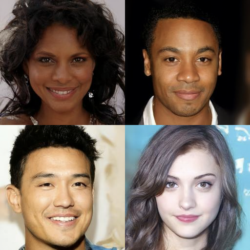
Four faces generated by DDPM on CelebA-HQ at 256x256 resolution (not cherry-picked). The iterative denoising approach produces photorealistic results competitive with GANs, but with stable training and no mode collapse (a GAN failure where the generator produces only a narrow subset of possible outputs).
Results. On unconditional CIFAR10 (32x32 images, 10 categories), DDPM achieves:
| Model | Inception Score | FID |
|---|---|---|
| StyleGAN2 + ADA | 9.74 | 3.26 |
| DDPM (\(L_\text{simple}\)) | 9.46 | 3.17 |
| NCSN | 8.87 | 25.32 |
FID (Frechet Inception Distance) measures how similar generated and real images are (lower is better). Inception Score measures quality and diversity (higher is better). DDPM achieves the best FID of any unconditional model, competitive even with models that use class labels (which DDPM does not).
The main limitation is sampling speed: generating one image requires 1000 sequential neural network evaluations. For 256x256 images, sampling a batch of 128 takes about 300 seconds, compared to a single forward pass for GANs.
Let us trace the complete sampling loop for a 1-pixel image with \(T = 3\) steps.
Given: \(\alpha_1 = 0.9\), \(\alpha_2 = 0.8\), \(\alpha_3 = 0.7\), so \(\bar{\alpha}_1 = 0.9\), \(\bar{\alpha}_2 = 0.72\), \(\bar{\alpha}_3 = 0.504\).
Set \(\sigma_t = \sqrt{\beta_t}\), so \(\sigma_3 = \sqrt{0.3} = 0.548\), \(\sigma_2 = \sqrt{0.2} = 0.447\), \(\sigma_1 = \sqrt{0.1} = 0.316\).
Start: Sample \(x_3 = 1.5\) from \(\mathcal{N}(0, 1)\).
Step \(t=3\): Network predicts \(\epsilon_\theta(1.5, 3) = 0.9\). Sample \(z = 0.3\).
\[x_2 = \frac{1}{\sqrt{0.7}} \left(1.5 - \frac{0.3}{\sqrt{0.496}} \times 0.9\right) + 0.548 \times 0.3\]
\[= 1.195 \times (1.5 - 0.426 \times 0.9) + 0.164 = 1.195 \times 1.117 + 0.164 = 1.335 + 0.164 = 1.499\]
Step \(t=2\): Network predicts \(\epsilon_\theta(1.499, 2) = 1.1\). Sample \(z = -0.5\).
\[x_1 = \frac{1}{\sqrt{0.8}} \left(1.499 - \frac{0.2}{\sqrt{0.28}} \times 1.1\right) + 0.447 \times (-0.5)\]
\[= 1.118 \times (1.499 - 0.378 \times 1.1) - 0.224 = 1.118 \times 1.083 - 0.224 = 1.211 - 0.224 = 0.987\]
Step \(t=1\): Network predicts \(\epsilon_\theta(0.987, 1) = 0.2\). Set \(z = 0\) (final step).
\[x_0 = \frac{1}{\sqrt{0.9}} \left(0.987 - \frac{0.1}{\sqrt{0.1}} \times 0.2\right) = 1.054 \times (0.987 - 0.316 \times 0.2) = 1.054 \times 0.924 = 0.974\]
Our generated “image” is \(x_0 = 0.974\). Starting from noise \(x_3 = 1.5\), the network’s denoising predictions guided us to a plausible data point.
Recall: Why does the sampling algorithm set \(z = 0\) at the final step (\(t = 1\)) but sample \(z \sim \mathcal{N}(0, I)\) at all other steps?
Apply: Given \(x_3 = -0.8\), \(\alpha_3 = 0.7\), \(\bar{\alpha}_3 = 0.504\), \(\sigma_3 = 0.548\), \(\epsilon_\theta = -0.4\), and \(z = 0.6\), compute \(x_2\).
Extend: DDPM requires 1000 network evaluations to generate one image. DDIM (a later method) showed that deterministic sampling with larger step sizes can reduce this to 50 steps. What trade-off would you expect between the number of sampling steps and image quality?
Describe the complete DDPM training loop in your own words. What are the inputs, what does the network predict, and what is the loss function?
Why does the paper fix the reverse process variance \(\sigma_t^2\) rather than learning it? What happened when the authors tried to learn it?
Both DDPM and GANs (see Generative Adversarial Nets) generate images, but through fundamentally different mechanisms. Compare the training procedure, generation speed, and training stability of the two approaches.
The simplified objective \(L_\text{simple}\) produces better FID but worse log-likelihood compared to the full variational bound. Why might this trade-off exist? What does the model “spend” its lossless coding capacity on?
DDPM uses the same core idea as VAEs (see Auto-Encoding Variational Bayes) – optimizing a variational lower bound on the data log-likelihood. What are the key structural differences? (Hint: consider the encoder, the latent space dimensionality, and whether the encoder is learned.)
Build a 1D diffusion model from scratch with numpy that learns to generate samples from a mixture of Gaussians.
The model should learn to generate samples clustered around \(-2\) and \(+2\), matching the bimodal data distribution.
import numpy as np

# --- Data ---
def sample_data(n):
    """Sample from mixture of two Gaussians: 0.5*N(-2,0.09) + 0.5*N(2,0.09)"""
    components = np.random.choice([-2.0, 2.0], size=n)
    return components + np.random.randn(n) * 0.3

# --- Noise schedule ---
T = 50
betas = np.linspace(1e-4, 0.02, T)
alphas = 1.0 - betas
alpha_bars = np.cumprod(alphas)  # cumulative product

# --- Simple MLP ---
def relu(x):
    return np.maximum(0, x)

def init_mlp(layer_sizes, seed=42):
    """Initialize MLP weights with Xavier initialization."""
    rng = np.random.RandomState(seed)
    params = []
    for i in range(len(layer_sizes) - 1):
        fan_in, fan_out = layer_sizes[i], layer_sizes[i + 1]
        scale = np.sqrt(2.0 / (fan_in + fan_out))
        W = rng.randn(fan_in, fan_out) * scale
        b = np.zeros(fan_out)
        params.append((W, b))
    return params

def forward_mlp(params, x):
    """Forward pass through MLP. ReLU on hidden layers, linear output."""
    for i, (W, b) in enumerate(params):
        x = x @ W + b
        if i < len(params) - 1:
            x = relu(x)
    return x

def backward_mlp(params, x, grad_output):
    """Backward pass. Returns gradients for each (W, b) pair."""
    # Forward pass storing activations
    activations = [x]
    for i, (W, b) in enumerate(params):
        x = x @ W + b
        if i < len(params) - 1:
            x = relu(x)
        activations.append(x)

    grads = []
    g = grad_output
    for i in reversed(range(len(params))):
        W, b = params[i]
        pre_act = activations[i] @ W + b
        if i < len(params) - 1:
            g = g * (pre_act > 0).astype(float)  # ReLU gradient
        grad_W = activations[i].T @ g / len(grad_output)
        grad_b = g.mean(axis=0)
        g = g @ W.T
        grads.append((grad_W, grad_b))

    return list(reversed(grads))

def timestep_embedding(t, dim=32):
    """Sinusoidal timestep embedding (same idea as Transformer position encoding)."""
    half = dim // 2
    freqs = np.exp(-np.log(1000.0) * np.arange(half) / half)
    args = t[:, None] * freqs[None, :]
    return np.concatenate([np.sin(args), np.cos(args)], axis=-1)

# --- TODO: Initialize the network ---
# Input: x_t (1 dim) concatenated with timestep embedding (32 dim) = 33 dims
# Hidden layers: 128, 128
# Output: predicted noise (1 dim)
# params = init_mlp([33, 128, 128, 1])

# --- TODO: Implement the forward diffusion shortcut ---
def q_sample(x_0, t, noise):
    """
    Compute x_t from x_0 using the closed-form formula.
    x_0: clean data, shape (batch,)
    t: timestep indices, shape (batch,), integers in [0, T-1]
    noise: epsilon, shape (batch,), sampled from N(0,1)
    Returns: x_t, shape (batch,)
    """
    pass  # TODO

# --- TODO: Implement noise prediction ---
def predict_noise(params, x_t, t):
    """
    Predict epsilon given noisy data x_t and timestep t.
    Concatenate x_t with timestep embedding and pass through MLP.
    x_t: shape (batch,)
    t: shape (batch,), integer timestep indices
    Returns: predicted noise, shape (batch,)
    """
    pass  # TODO

# --- TODO: Implement one training step ---
def train_step(params, x_0, lr=1e-3):
    """
    One step of L_simple training.
    1. Sample random timesteps
    2. Sample noise
    3. Compute x_t using q_sample
    4. Predict noise
    5. Compute MSE loss
    6. Backpropagate and update params
    Returns: updated params, loss value
    """
    pass  # TODO

# --- TODO: Implement the sampling loop ---
def sample(params, n_samples):
    """
    Generate samples by running the full reverse process.
    1. Start from x_T ~ N(0, 1)
    2. For t = T-1, ..., 0:
       - Predict noise
       - Compute x_{t-1} using the reverse step formula
       - Add noise z if t > 0
    Returns: generated samples, shape (n_samples,)
    """
    pass  # TODO

# --- Training loop ---
# params = init_mlp([33, 128, 128, 1])
# for step in range(5000):
#     x_0 = sample_data(256)
#     params, loss = train_step(params, x_0)
#     if step % 500 == 0:
#         print(f"Step {step}, Loss: {loss:.4f}")
#
# --- Generate and verify ---
# samples = sample(params, 1000)
# print(f"Sample mean: {samples.mean():.2f} (expect ~0.0)")
# print(f"Sample std:  {samples.std():.2f} (expect ~2.1)")
# print(f"Fraction near -2: {((samples > -3) & (samples < -1)).mean():.2f} (expect ~0.50)")
# print(f"Fraction near +2: {((samples > 1) & (samples < 3)).mean():.2f} (expect ~0.50)")Step 0, Loss: 1.0234
Step 500, Loss: 0.4812
Step 1000, Loss: 0.3156
Step 1500, Loss: 0.2843
Step 2000, Loss: 0.2501
Step 2500, Loss: 0.2295
Step 3000, Loss: 0.2187
Step 3500, Loss: 0.2098
Step 4000, Loss: 0.2034
Step 4500, Loss: 0.1967
Sample mean: -0.05 (expect ~0.0)
Sample std: 2.14 (expect ~2.1)
Fraction near -2: 0.48 (expect ~0.50)
Fraction near +2: 0.49 (expect ~0.50)The generated samples should cluster around \(-2\) and \(+2\), matching the bimodal training distribution. The loss values are approximate – exact numbers depend on random seeds, but the loss should decrease steadily and the generated samples should clearly show two modes.