Improving Language Understanding by Generative Pre-Training: Course

Learning Objectives

By the end of this course, you will be able to:

1. Explain why pre-training on unlabeled text solves the labeled data bottleneck for NLP (natural language processing) tasks
2. Compute the language modeling objective (next-token prediction) by hand for a short sequence
3. Describe how GPT adapts the Transformer decoder for left-to-right language modeling
4. Walk through fine-tuning: adding a linear head and training on labeled data
5. Convert structured NLP tasks (entailment, similarity, multiple choice) into token sequences using GPT’s input transformations
6. Explain why an auxiliary language modeling loss during fine-tuning improves generalization

Prerequisites

• Python and numpy – you should be comfortable writing functions, loops, and working with numpy arrays
• Basic probability – probability distributions, conditional probability, log-likelihood. You should know that \(\log(ab) = \log(a) + \log(b)\) and that maximizing log-probability is equivalent to maximizing probability.
• Softmax function – converts a vector of raw scores into a probability distribution. Covered in the Transformer course.
• Matrix multiplication – you should know that multiplying an \((n \times d)\) matrix by a \((d \times m)\) matrix produces an \((n \times m)\) matrix
• The Transformer architecture – self-attention, multi-head attention, feed-forward networks, residual connections, and layer normalization. You should have completed the Transformer course (see Attention Is All You Need).
• Generative models – the concept that models can learn to produce data by modeling a probability distribution. The GAN and VAE courses provide this foundation (see Generative Adversarial Nets and Auto-Encoding Variational Bayes).

Lesson 1: The Labeled Data Problem

Before GPT, every NLP task required a custom model trained on task-specific labeled data. This lesson explains why that was a dead end and what insight led to the solution.

Explanation

Imagine you want to build four separate systems: one that answers questions about documents, one that detects whether a movie review is positive or negative, one that decides if two sentences mean the same thing, and one that determines if a hypothesis follows from a premise. Before GPT, the standard approach was to collect thousands of hand-labeled examples for each task, design a task-specific architecture for each one, and train four completely independent models.

This has three problems:

Problem 1: Labeling is expensive. A human must read each example and assign the correct answer. For question answering, someone must read a passage and write the answer. For sentiment analysis, someone must read a review and decide positive or negative. Getting 10,000 labels per task across four tasks means 40,000 human judgments. For many languages and specialized domains, labeled data simply does not exist.

Problem 2: Knowledge is not shared. The sentiment model learns nothing from the question-answering data. Each model starts from scratch. But language understanding is largely shared – grammar, word meanings, reasoning patterns, and world knowledge are the same regardless of the task.

Problem 3: Small datasets produce fragile models. A model trained on 2,500 examples (like the RTE entailment dataset) cannot learn general language understanding – it memorizes surface patterns instead. It might learn that sentences containing “not” are likely contradictions, rather than truly understanding negation.

The insight behind GPT is borrowed from how humans learn language. A child does not learn to read by studying labeled examples of sentiment analysis. They learn by reading – absorbing grammar, vocabulary, reasoning patterns, and world knowledge from massive amounts of text. Only after building this foundation do they learn specific skills like essay writing or test-taking, requiring relatively little targeted practice.

Transfer learning formalizes this idea. Train a model on a large, general task first (pre-training), then adapt it to specific tasks with small amounts of labeled data (fine-tuning). The key question is: what general task teaches the most useful knowledge?

Worked Example

Consider the sentence: “The bank by the river was steep and covered in wildflowers.”

A model that truly understands language should know:

• “bank” here means riverbank, not financial institution (disambiguation)
• “steep” describes the angle of the bank (adjective-noun relationship)
• “wildflowers” grow on natural surfaces (world knowledge)
• This sentence describes a natural scene (inference)

Now consider three NLP tasks using this sentence:

Sentiment analysis: “The bank by the river was steep and covered in wildflowers.” – Positive or negative? The model needs to recognize “wildflowers” as pleasant imagery.

Entailment: Premise: “The bank by the river was steep and covered in wildflowers.” Hypothesis: “There were flowers near the water.” – The model needs to know that a river has water, wildflowers are flowers, and “by the river” means “near the water.”

Similarity: “The bank by the river was steep and covered in wildflowers” vs. “The hillside along the stream was angled and full of wild plants.” – The model needs to recognize synonyms (bank/hillside, river/stream) and paraphrases.

All three tasks require the same underlying knowledge: word meanings, grammar, and reasoning. Training three separate models from scratch would force each to re-learn all of this from limited labeled data. Pre-training lets a single model learn this shared knowledge once, then each task benefits from it.

Exercises

Recall: What are the three problems with training a separate model for each NLP task from scratch? Which problem does pre-training primarily solve?

Apply: You have 500 labeled examples for a medical question-answering task and access to 10 million unlabeled medical research papers. Describe a two-stage approach using transfer learning. What does the model learn in each stage?

Extend: Word embeddings (like Word2Vec) also transfer knowledge from unlabeled text. But GPT was a major improvement over word embeddings. What kind of knowledge can a language model capture that individual word embeddings cannot? (Hint: think about word order, sentence structure, and multi-sentence reasoning.)

Lesson 2: Language Modeling – Learning by Prediction

GPT pre-trains by predicting the next word in a sequence. This lesson explains why next-word prediction is such a powerful learning signal and formalizes it mathematically.

Explanation

Think of a game where you cover up the last word of a sentence and try to guess it. Given “The cat sat on the ___”, you would guess “mat” or “floor” or “couch” – something that makes sense as a surface a cat would sit on. To play this game well, you need to understand grammar (what part of speech fits here), semantics (cats sit on surfaces), and world knowledge (common surfaces).

Language modeling is exactly this game, played at industrial scale. The model reads millions of sentences and, for each position, predicts the next token given all previous tokens. The training objective maximizes the probability the model assigns to the actual next tokens:

\[L_1(\mathcal{U}) = \sum_{i} \log P(u_i \mid u_{i-k}, \ldots, u_{i-1}; \Theta)\]

• \(\mathcal{U} = \{u_1, \ldots, u_n\}\): the corpus of unlabeled tokens (for GPT, over 7,000 books)
• \(u_i\): the \(i\)-th token in the corpus
• \(k\): the context window size (512 tokens in GPT – roughly one page of text)
• \(P(u_i \mid u_{i-k}, \ldots, u_{i-1}; \Theta)\): the probability the model assigns to token \(u_i\) given the preceding \(k\) tokens
• \(\Theta\): all the model’s learnable parameters (weights and biases)

Why log-probability? The probability of a sequence is the product of individual token probabilities: \(P(u_1, u_2, u_3) = P(u_1) \cdot P(u_2 | u_1) \cdot P(u_3 | u_1, u_2)\). Products of many small numbers become numerically tiny (underflow). Taking the log converts products into sums: \(\log P = \log P(u_1) + \log P(u_2|u_1) + \log P(u_3|u_1, u_2)\). Sums are numerically stable and easier to optimize.

Why this objective works so well: Consider what the model must learn to predict the next word in different contexts:

• “The capital of France is ___” → “Paris” (factual knowledge)
• “She picked up the phone and ___” → “called” or “dialed” (common actions)
• “Despite the rain, the picnic was ___” → “enjoyable” or “fun” (reasoning about contrast)
• “The doctor told the patient that she ___” → requires resolving “she” (coreference)

Each of these predictions requires a different kind of understanding. Across billions of predictions on diverse text, the model is forced to build internal representations that capture grammar, semantics, factual knowledge, and reasoning – all as a side effect of next-word prediction.

Worked Example

Let’s compute the language modeling loss for the sentence “The cat sat” using a tiny vocabulary of 5 tokens: {the, cat, sat, dog, on}.

Suppose the model produces these probability distributions:

Position 1: predict “cat” given [“The”]

The correct token is “cat” with probability 0.40.

\(\log P(\text{cat} \mid \text{The}) = \log(0.40) = -0.916\)

Position 2: predict “sat” given [“The”, “cat”]

The correct token is “sat” with probability 0.60.

\(\log P(\text{sat} \mid \text{The, cat}) = \log(0.60) = -0.511\)

Total loss (to maximize):

\[L_1 = \log P(\text{cat} \mid \text{The}) + \log P(\text{sat} \mid \text{The, cat}) = -0.916 + (-0.511) = -1.427\]

A perfect model would assign probability 1.0 to each correct token, giving \(L_1 = \log(1) + \log(1) = 0\). Our model’s loss of \(-1.427\) reflects uncertainty – training pushes the model to assign higher probability to the correct tokens.

Perplexity is a more intuitive metric. It measures how “surprised” the model is, on average, by each token:

\[\text{Perplexity} = e^{-L_1 / N} = e^{-(-1.427) / 2} = e^{0.714} = 2.04\]

A perplexity of 2.04 means the model is, on average, as uncertain as choosing between 2 equally likely options. The GPT paper achieved a perplexity of 18.4 on BooksCorpus – as uncertain as choosing between roughly 18 options out of a 40,000-token vocabulary. That’s remarkably good.

Exercises

Recall: Why does GPT use log-probability instead of raw probability in its training objective? What numerical problem does this avoid?

Apply: A model predicts the next token in “I love ___” and assigns these probabilities: {cats: 0.30, dogs: 0.25, pizza: 0.20, sleep: 0.15, rocks: 0.10}. The actual next word is “cats.” Compute the log-probability. Then compute the perplexity for this single prediction.

Extend: GPT pre-trains on BooksCorpus (over 7,000 books). The paper specifically chose books over the 1 Billion Word Benchmark, which is shuffled at the sentence level. Why would shuffled sentences hurt pre-training, even if the total word count is similar? What kind of knowledge requires long, coherent passages?

Lesson 3: The Decoder-Only Architecture

GPT uses the decoder half of the Transformer architecture from “Attention Is All You Need.” This lesson explains what “decoder-only” means, how masked self-attention enforces left-to-right processing, and how the model converts hidden states into word predictions.

Explanation

Recall from the Transformer course that the original Transformer has two parts: an encoder (which reads the full input) and a decoder (which generates output one token at a time). The encoder uses bidirectional attention – each position can attend to every other position. The decoder uses masked attention – each position can only attend to itself and earlier positions.

GPT makes a bold simplification: it throws away the encoder entirely and uses only the decoder. Why? Because language modeling is inherently left-to-right. When predicting the next word in “The cat sat on the ___”, the model should only use information from the words that come before the blank – not after it. Masked self-attention enforces exactly this constraint.

The full computation has three stages:

\[h_0 = U W_e + W_p\]

\[h_l = \text{transformer\_block}(h_{l-1}) \quad \forall \, l \in [1, n]\]

\[P(u) = \text{softmax}(h_n W_e^T)\]

• \(U = (u_{-k}, \ldots, u_{-1})\): the context vector of token indices
• \(W_e\): the token embedding matrix, shape (vocabulary size \(\times\) 768). Each row is the 768-dimensional vector for one token.
• \(W_p\): the position embedding matrix, shape (512 \(\times\) 768). Each row encodes a position in the sequence.
• \(h_0\): the initial hidden state after combining token and position embeddings
• \(h_l\): the hidden state after the \(l\)-th Transformer block
• \(n\): the number of Transformer layers (12 in GPT)
• \(W_e^T\): the transposed embedding matrix, reused for the output projection
• \(\text{softmax}(h_n W_e^T)\): the final probability distribution over the vocabulary

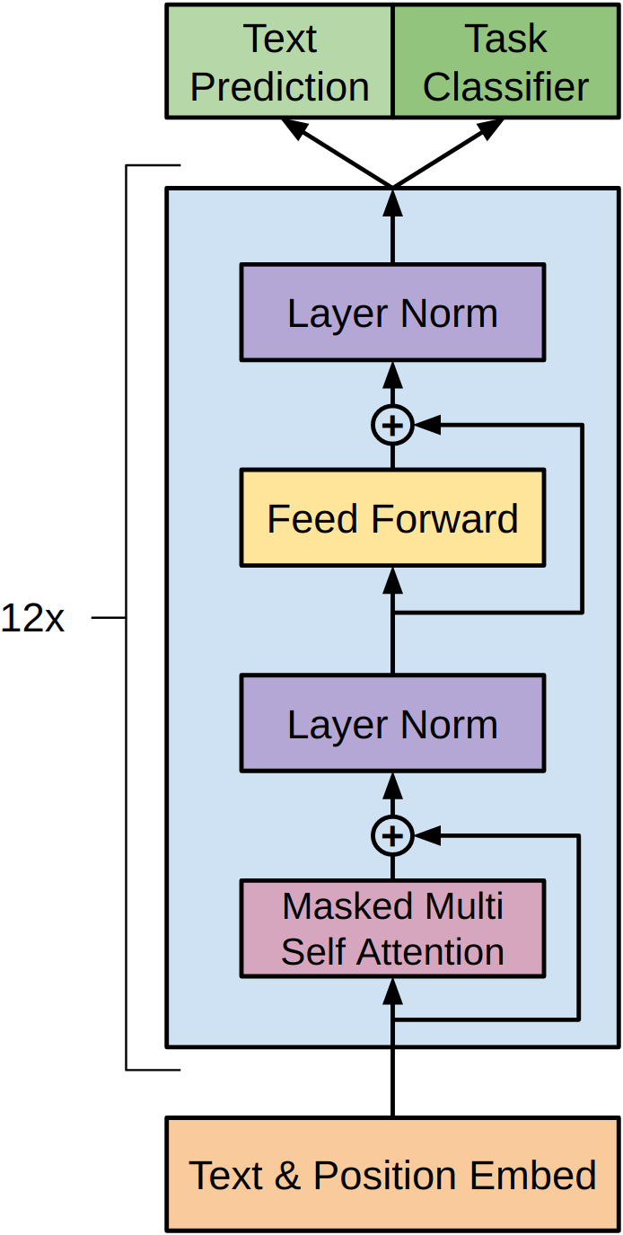
Stage 1: Embed. Each token is looked up in \(W_e\) to get a 768-dimensional vector. A separate position embedding from \(W_p\) is added. Unlike the original Transformer’s sinusoidal position encodings (which are fixed mathematical functions), GPT uses learned position embeddings – the model discovers the best way to encode position during training.

Stage 2: Transform. The embedded sequence passes through 12 identical Transformer blocks. Each block contains masked multi-head self-attention (12 heads, each working in 64 dimensions) followed by a feed-forward network (expanding from 768 to 3072, then compressing back to 768). Each sub-layer is wrapped with a residual connection and layer normalization. The activation function is GELU (Gaussian Error Linear Unit) instead of the original Transformer’s ReLU.

Stage 3: Predict. The final hidden state \(h_{12}\) is multiplied by the transpose of the embedding matrix \(W_e^T\) to produce a score for every token in the vocabulary. Softmax converts these scores to probabilities.

Figure 1: The GPT architecture. Input tokens are converted to embeddings and combined with position embeddings at the bottom. These pass through 12 identical Transformer blocks, each containing masked multi-head self-attention and a feed-forward network with residual connections and layer normalization. The top produces two outputs: a text prediction head (for the language modeling objective) and a task classifier head (for the downstream task during fine-tuning).

Weight tying: notice that \(W_e\) is used twice – once to convert tokens into vectors (input), and once transposed to convert vectors back into token scores (output). This technique, called weight tying, reduces the parameter count and forces the embeddings to work well for both understanding and prediction. If “cat” and “kitten” have similar embeddings (because they appear in similar contexts), then the model will assign similar probabilities to both when either is a plausible next word.

Worked Example

Let’s trace the forward pass for a 3-token sequence [“I”, “love”, “cats”] with a tiny model: vocabulary size = 5, \(d_\text{model} = 4\), 1 Transformer layer.

Token indices: I=0, love=1, cats=2, dogs=3, the=4.

Embedding matrix \(W_e\) (5 \(\times\) 4):

\[W_e = \begin{bmatrix} 0.2 & -0.1 & 0.5 & 0.3 \\ 0.8 & 0.4 & -0.2 & 0.1 \\ 0.1 & 0.7 & 0.3 & -0.4 \\ 0.3 & 0.6 & 0.2 & -0.3 \\ -0.5 & 0.2 & 0.4 & 0.6 \end{bmatrix}\]

Position embedding \(W_p\) (3 \(\times\) 4):

\[W_p = \begin{bmatrix} 0.0 & 0.1 & 0.0 & -0.1 \\ 0.1 & 0.0 & -0.1 & 0.1 \\ 0.0 & -0.1 & 0.1 & 0.0 \end{bmatrix}\]

Stage 1: Look up token embeddings and add position embeddings.

• “I” (token 0, position 0): \([0.2, -0.1, 0.5, 0.3] + [0.0, 0.1, 0.0, -0.1] = [0.2, 0.0, 0.5, 0.2]\)
• “love” (token 1, position 1): \([0.8, 0.4, -0.2, 0.1] + [0.1, 0.0, -0.1, 0.1] = [0.9, 0.4, -0.3, 0.2]\)
• “cats” (token 2, position 2): \([0.1, 0.7, 0.3, -0.4] + [0.0, -0.1, 0.1, 0.0] = [0.1, 0.6, 0.4, -0.4]\)

\[h_0 = \begin{bmatrix} 0.2 & 0.0 & 0.5 & 0.2 \\ 0.9 & 0.4 & -0.3 & 0.2 \\ 0.1 & 0.6 & 0.4 & -0.4 \end{bmatrix}\]

Stage 2: Pass through the masked Transformer block. The masking ensures:

• “I” (position 0) attends only to itself
• “love” (position 1) attends to “I” and itself
• “cats” (position 2) attends to “I”, “love”, and itself

After one Transformer block (attention + FFN + residuals + layer norm), suppose \(h_1\) is:

\[h_1 = \begin{bmatrix} -0.8 & 1.2 & 0.3 & -0.7 \\ 0.5 & -0.3 & 1.1 & -1.3 \\ -0.2 & 0.9 & -1.0 & 0.3 \end{bmatrix}\]

Stage 3: Compute output scores. Multiply \(h_1\) by \(W_e^T\) (shape \(4 \times 5\)):

For “cats” (position 2, the last position), \(h_1[2] = [-0.2, 0.9, -1.0, 0.3]\):

\[h_1[2] \cdot W_e^T = \begin{bmatrix} -0.2 \times 0.2 + 0.9 \times (-0.1) + (-1.0) \times 0.5 + 0.3 \times 0.3 \\ -0.2 \times 0.8 + 0.9 \times 0.4 + (-1.0) \times (-0.2) + 0.3 \times 0.1 \\ -0.2 \times 0.1 + 0.9 \times 0.7 + (-1.0) \times 0.3 + 0.3 \times (-0.4) \\ -0.2 \times 0.3 + 0.9 \times 0.6 + (-1.0) \times 0.2 + 0.3 \times (-0.3) \\ -0.2 \times (-0.5) + 0.9 \times 0.2 + (-1.0) \times 0.4 + 0.3 \times 0.6 \end{bmatrix}^T\]

Computing each score:

• I: \(-0.04 - 0.09 - 0.50 + 0.09 = -0.54\)
• love: \(-0.16 + 0.36 + 0.20 + 0.03 = 0.43\)
• cats: \(-0.02 + 0.63 - 0.30 - 0.12 = 0.19\)
• dogs: \(-0.06 + 0.54 - 0.20 - 0.09 = 0.19\)
• the: \(0.10 + 0.18 - 0.40 + 0.18 = 0.06\)

Scores: \([-0.54, 0.43, 0.19, 0.19, 0.06]\)

After softmax: \(P = [0.098, 0.259, 0.204, 0.204, 0.179]\)

The model predicts “love” (25.9%) is the most likely next word after “I love cats.” Notice that “cats” and “dogs” get equal scores (0.19 each) – their embeddings are similar, and the model hasn’t trained enough to distinguish which is more likely here.

Exercises

Recall: Why does GPT use only the decoder half of the Transformer, not the encoder-decoder? What constraint does masked self-attention enforce, and why is it necessary for language modeling?

Apply: GPT has a vocabulary of 40,000 tokens, embedding dimension 768, and 512 positions. How many parameters are in \(W_e\) and \(W_p\) combined? The weight tying trick reuses \(W_e\) at the output – how many parameters does this save compared to having a separate output projection matrix?

Extend: The original Transformer uses sinusoidal position encodings (fixed mathematical formulas), while GPT uses learned position embeddings. What is the advantage of learned embeddings? What is the disadvantage? (Hint: think about what happens when the model encounters a sequence longer than 512 tokens at test time.)

Lesson 4: Fine-Tuning with a Linear Head

Pre-training gives us a model that understands language. Fine-tuning adapts it to a specific task. This lesson covers how GPT adds a task-specific output layer and trains on labeled data.

Explanation

Think of hiring a brilliant writer who has read thousands of books and asking them to become a movie reviewer. You don’t need to teach them English – they already know grammar, vocabulary, and how to reason about narratives. You just need to show them a few hundred movie reviews with star ratings, and they quickly learn the format: read a review, output a rating.

Fine-tuning works the same way. The pre-trained GPT model already understands language deeply. To adapt it for a task like sentiment classification, we add a single new layer on top and train on labeled examples.

The fine-tuning objective is:

\[L_2(\mathcal{C}) = \sum_{(x,y)} \log P(y \mid x_1, \ldots, x_m)\]

• \(\mathcal{C}\): the labeled dataset for the target task
• \((x, y)\): a training example with input tokens \(x_1, \ldots, x_m\) and label \(y\)
• \(P(y \mid x_1, \ldots, x_m)\): the probability of label \(y\) given the input

The prediction is computed as:

\[P(y \mid x_1, \ldots, x_m) = \text{softmax}(h_l^m W_y)\]

• \(h_l^m\): the final Transformer layer’s output at the last token position \(m\)
• \(W_y\): a new learned linear projection matrix, shape (768 \(\times\) number of classes)

This is the only new component. For a 3-class sentiment task (positive, neutral, negative), \(W_y\) has shape \(768 \times 3\), adding just 2,304 new parameters to the 117 million pre-trained parameters.

Why the last token position? In a decoder with masked attention, each position’s representation captures information from all preceding positions. The last position has seen the entire input, so its hidden state is the richest summary of the full sequence. Using it as the “sentence representation” is natural for a left-to-right model.

How fine-tuning updates the model: During fine-tuning, all parameters are updated – both the new linear layer \(W_y\) and all 12 pre-trained Transformer layers. The pre-trained weights are not frozen. But because they start from a good initialization (the pre-trained values), the model converges quickly – just 3 epochs (complete passes through the training data) of training in most cases. The learning rate is lower than during pre-training (\(6.25 \times 10^{-5}\) vs. \(2.5 \times 10^{-4}\)) to avoid large updates that could destroy the pre-trained knowledge.

What changes, what stays: The paper’s ablation study (an experiment that removes one component at a time to measure its contribution) showed that removing pre-training caused a 14.8% average performance drop. Replacing the Transformer with an LSTM (Long Short-Term Memory, a recurrent network that processes tokens one at a time in sequence) while keeping everything else identical caused a 5.6% drop. This tells us that both the pre-trained knowledge and the Transformer architecture are essential, but pre-training is the dominant factor.

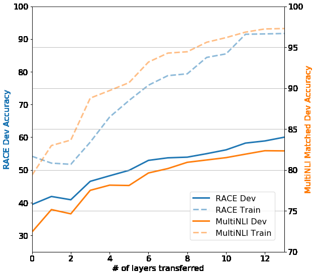
Figure 2: Effect of transferring different numbers of pre-trained layers. Zero layers means only the embeddings are transferred. Each additional layer improves performance, with gains continuing all the way to the full 12 layers. This suggests every layer captures useful knowledge – earlier layers likely encode syntax, while deeper layers capture more abstract semantic and reasoning patterns.

Worked Example

Let’s trace fine-tuning for a binary sentiment task (positive/negative) with a toy 4-dimensional model.

Input: “I love cats” (3 tokens, already embedded and processed through the Transformer as in Lesson 3).

After the Transformer, the hidden state at the last position (“cats”) is:

\[h_l^m = [-0.2, 0.9, -1.0, 0.3]\]

New linear layer \(W_y\) (shape \(4 \times 2\), randomly initialized):

\[W_y = \begin{bmatrix} 0.15 & -0.20 \\ 0.30 & 0.10 \\ -0.25 & 0.40 \\ 0.10 & -0.15 \end{bmatrix}\]

Compute logits (raw scores for each class):

\[h_l^m W_y = [-0.2, 0.9, -1.0, 0.3] \begin{bmatrix} 0.15 & -0.20 \\ 0.30 & 0.10 \\ -0.25 & 0.40 \\ 0.10 & -0.15 \end{bmatrix}\]

• Positive: \((-0.2)(0.15) + (0.9)(0.30) + (-1.0)(-0.25) + (0.3)(0.10) = -0.03 + 0.27 + 0.25 + 0.03 = 0.52\)
• Negative: \((-0.2)(-0.20) + (0.9)(0.10) + (-1.0)(0.40) + (0.3)(-0.15) = 0.04 + 0.09 - 0.40 - 0.045 = -0.315\)

Logits: \([0.52, -0.315]\)

Softmax:

\[e^{0.52} = 1.682, \quad e^{-0.315} = 0.730\]

\[P(\text{positive}) = \frac{1.682}{1.682 + 0.730} = 0.697, \quad P(\text{negative}) = \frac{0.730}{2.412} = 0.303\]

The model predicts 69.7% positive. If the true label is positive:

\[L_2 = \log P(\text{positive}) = \log(0.697) = -0.361\]

The gradient of this loss flows back through \(W_y\) and through all 12 Transformer layers, nudging the entire model to produce hidden states that lead to correct classifications.

Exercises

Recall: Why does GPT use the hidden state at the last token position as the input to the classifier, rather than averaging all positions? What property of masked attention makes the last position special?

Apply: A pre-trained GPT model is fine-tuned for a 4-class task (entailment, contradiction, neutral, unrelated). The model has 768-dimensional hidden states. How many parameters does the new linear layer \(W_y\) add? What percentage of GPT’s 117 million total parameters is this?

Extend: The fine-tuning learning rate (\(6.25 \times 10^{-5}\)) is 4x smaller than the pre-training learning rate (\(2.5 \times 10^{-4}\)). Why use a smaller learning rate? What would happen if you used the same large learning rate? What would happen if you froze the pre-trained weights entirely and only trained \(W_y\)?

Lesson 5: Task-Specific Input Transformations

GPT is pre-trained on plain text sequences, but many NLP tasks have structured inputs: premise-hypothesis pairs, question-document-answer triples, or sentence pairs. This lesson covers GPT’s clever trick for handling them all without changing the architecture.

Explanation

Imagine you have a machine that reads a single continuous stream of text and produces a summary at the end. Now you want it to compare two documents. You could build a new machine with two input slots – or you could just put both documents into the same stream with a clear separator between them: “[Document A] — [Document B]”. The machine reads the combined stream and its summary at the end captures information about both documents and their relationship.

GPT uses exactly this approach. Special tokens act as separators and markers:

• [Start]: marks the beginning of the input
• [Delim]: separates different parts of the input (delimiter)
• [Extract]: marks the end – the hidden state at this position is used for classification

The model learns embeddings for these special tokens during fine-tuning. These are among the very few new parameters added (3 new token embeddings \(\times\) 768 dimensions = 2,304 parameters).

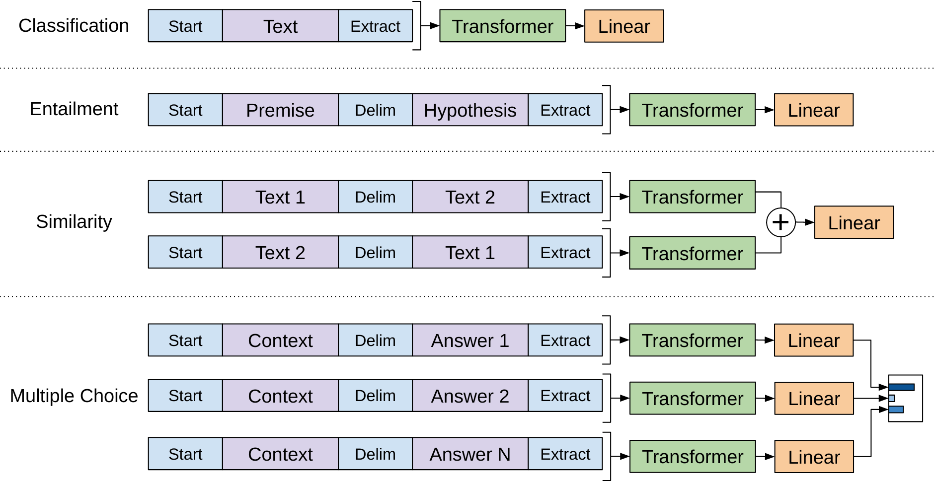
Figure 3: How GPT handles four different task types without changing the model architecture. Classification: the text is wrapped with Start and Extract tokens. Entailment: premise and hypothesis are concatenated with a Delim token. Similarity: both orderings are processed and their representations added. Multiple Choice: each answer is concatenated with the context and compared via softmax.

Here is how each task type is formatted:

Classification (e.g., sentiment analysis): the simplest case. Wrap the input text with special tokens.

Input: [Start] This movie was absolutely wonderful [Extract]

The hidden state at the [Extract] position is fed to the linear classifier.

Entailment (e.g., does the hypothesis follow from the premise?): concatenate premise and hypothesis with a delimiter.

Input: [Start] A man is playing guitar on stage [Delim] A musician is performing [Extract]

The model processes both sentences as a single sequence. Because each position attends to all previous positions, the hypothesis tokens can attend to the premise tokens. The [Extract] hidden state captures the relationship.

Similarity (e.g., are two sentences paraphrases?): similarity is symmetric – “A is similar to B” should equal “B is similar to A.” But masked attention is not symmetric – the second sentence can attend to the first, but not vice versa. The solution: process both orderings and add the results.

Order 1: [Start] The cat sat on the mat [Delim] A feline rested on a rug [Extract] Order 2: [Start] A feline rested on a rug [Delim] The cat sat on the mat [Extract]

Each ordering produces a hidden state at [Extract]. These two vectors are added element-wise, and the sum is fed to the classifier.

Multiple Choice (e.g., question answering with answer options): concatenate the context with each answer option separately, process each independently, and compare via softmax.

Option A: [Start] The cat was hungry. What did it do? [Delim] It ate some food [Extract] Option B: [Start] The cat was hungry. What did it do? [Delim] It went swimming [Extract] Option C: [Start] The cat was hungry. What did it do? [Delim] It read a book [Extract]

Each option produces a scalar score from the linear layer. Softmax across the three scores gives probabilities: the highest-probability answer wins.

Worked Example

Let’s trace the entailment input transformation for a concrete example from the MultiNLI dataset.

Task: Given a premise and hypothesis, classify as entailment, contradiction, or neutral.

Premise: “The old man spoke to the young girl” Hypothesis: “An elderly person talked to a child”

Step 1: Tokenize (using BPE – Byte Pair Encoding, a method that builds a vocabulary by iteratively merging the most frequent character pairs – with 40,000 merges). Simplified for clarity:

Premise tokens: [“The”, “old”, “man”, “spoke”, “to”, “the”, “young”, “girl”] Hypothesis tokens: [“An”, “elderly”, “person”, “talked”, “to”, “a”, “child”]

Step 2: Apply input transformation:

Full sequence: [“[Start]”, “The”, “old”, “man”, “spoke”, “to”, “the”, “young”, “girl”, “[Delim]”, “An”, “elderly”, “person”, “talked”, “to”, “a”, “child”, “[Extract]”]

Token count: 19 tokens (well within the 512-token context window).

Step 3: Embed. Each token gets its embedding from \(W_e\) (or the newly learned embedding for [Start], [Delim], [Extract]). Position embeddings from \(W_p\) are added for positions 0 through 18.

Step 4: Process through 12 Transformer layers. The masking ensures:

• “spoke” (position 4) can attend to “The”, “old”, “man”, “spoke” – but not to any hypothesis tokens
• “talked” (position 13) can attend to all premise tokens and “An”, “elderly”, “person”, “talked” – it can see the premise and draw comparisons
• “[Extract]” (position 18) can attend to everything – it sees the full premise and hypothesis

Step 5: Classify. The hidden state at position 18 ([Extract]) is multiplied by \(W_y\) (shape \(768 \times 3\)) and passed through softmax:

\[P(\text{entailment}) = 0.82, \quad P(\text{neutral}) = 0.14, \quad P(\text{contradiction}) = 0.04\]

The model correctly identifies this as entailment – “elderly person” entails “old man” and “talked to” entails “spoke to.”

Exercises

Recall: Why does the similarity task process both orderings of the sentence pair? What property of masked attention creates an asymmetry that needs to be corrected?

Apply: Format the following multiple choice question for GPT input. Context: “Marie Curie discovered radium in 1898.” Question: “What element did Curie discover?” Options: (A) Uranium, (B) Radium, (C) Polonium. Write out the three input sequences using [Start], [Delim], and [Extract] tokens.

Extend: The input transformations convert structured inputs into flat token sequences, avoiding any architectural changes. An alternative approach (used by some pre-GPT models) is to encode each input piece with a separate encoder and combine the representations. What are the advantages of GPT’s flat-sequence approach? What information might be lost compared to separate encoding? (Hint: think about cross-attention between premise and hypothesis tokens.)

Lesson 6: The Pre-Train-Then-Fine-Tune System

This final lesson brings everything together: pre-training, the decoder architecture, fine-tuning, input transformations, and a final ingredient – the auxiliary language modeling loss that acts as a regularizer during fine-tuning. This complete system is GPT’s main contribution.

Explanation

We have all the pieces. Let’s assemble the full pipeline and understand the one remaining component: the combined training objective during fine-tuning.

The complete GPT pipeline:

1. Pre-train a 12-layer Transformer decoder on BooksCorpus (7,000+ books, ~800 million words) using the language modeling objective \(L_1\) for 100 epochs
2. Format the task input using the appropriate transformation (Lesson 5)
3. Add a linear classification head on top of the pre-trained model
4. Fine-tune on labeled data for 3 epochs using the combined objective \(L_3\)

The combined objective is:

\[L_3(\mathcal{C}) = L_2(\mathcal{C}) + \lambda \cdot L_1(\mathcal{C})\]

• \(L_2(\mathcal{C})\): the supervised classification loss (Lesson 4)
• \(L_1(\mathcal{C})\): the language modeling loss computed on the fine-tuning data (next-token prediction)
• \(\lambda = 0.5\): a weighting coefficient

Why add language modeling during fine-tuning? The classification loss \(L_2\) alone would update all 117 million parameters to optimize for the specific task. With a small dataset (say, 5,000 examples), this creates a risk: the model overfits to the task data and loses its general language understanding – a phenomenon called catastrophic forgetting. The pre-trained weights drift far from their useful initial values.

Adding \(L_1\) as an auxiliary loss acts as a regularizer. It says: “while you’re learning to classify, keep being a good language model too.” This anchors the weights closer to their pre-trained values, preserving the general knowledge while still learning the task. The paper found this is particularly beneficial for larger datasets, where the model trains for more total steps and has more opportunity to drift.

The ablation evidence: Removing the auxiliary \(L_1\) during fine-tuning dropped average performance by about 0.3 points. The effect was larger on bigger datasets (like MultiNLI with 392,000 examples) and smaller on tiny datasets (like RTE with 2,490 examples). This makes sense: with very few examples, the model barely updates anyway, so there’s less drift to prevent.

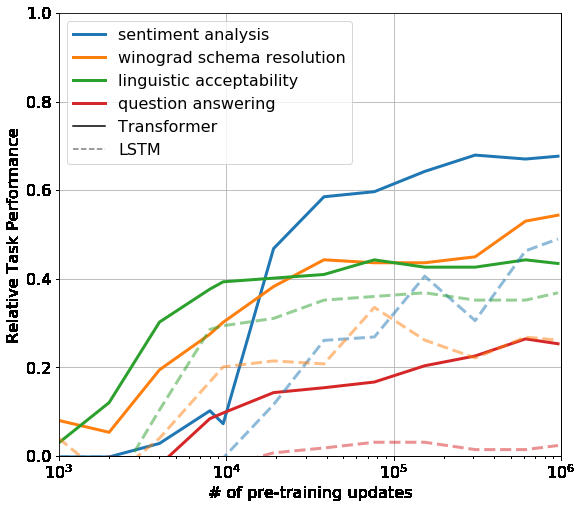
Figure 4: Zero-shot task performance (no fine-tuning) as a function of pre-training updates. Solid lines are the Transformer, dashed lines are an LSTM. The Transformer steadily improves on all tasks as pre-training progresses, while the LSTM shows higher variance and lower overall performance. This demonstrates that the Transformer learns task-relevant capabilities as a side effect of language modeling – even before any fine-tuning.

Results and what they proved: GPT achieved state-of-the-art results on 9 out of 12 tasks, often beating ensemble models (combinations of 3-5 models) with a single model. The most impressive results were:

• Story Cloze: 86.5% (previous best: 77.6%) – requires understanding narrative structure
• RACE reading comprehension: 59.0% (previous best: 53.3%) – requires multi-sentence reasoning
• MultiNLI: 82.1% (previous best: 80.6% with a 3-model ensemble) – requires logical inference

The one weak spot was RTE (56.0% vs. 61.7% for a BiLSTM baseline). RTE has only 2,490 training examples – too few for the large model to adapt properly. This foreshadowed a pattern: GPT-style models need enough fine-tuning data to steer the large pre-trained model, or they need to be bigger so they can learn from fewer examples (as GPT-3 later demonstrated with in-context learning).

Why this was a paradigm shift: Before GPT, each NLP task required a custom architecture. After GPT, the recipe was simple: one architecture, one pre-training run, minimal adaptation per task. This is the “pre-train then fine-tune” paradigm that became the foundation for BERT, GPT-2, GPT-3, and ultimately ChatGPT.

Worked Example

Let’s trace the combined loss computation for one fine-tuning example.

Task: Sentiment classification (positive/negative) Input: “This film was brilliant” → tokens: [Start, This, film, was, brilliant, Extract] Label: positive (\(y = 1\))

Step 1: Compute the classification loss \(L_2\).

The Transformer processes all 6 tokens. The hidden state at “Extract” (position 5) passes through \(W_y\) (shape \(768 \times 2\)):

Suppose the model outputs: \(P(\text{positive}) = 0.85\), \(P(\text{negative}) = 0.15\).

\[L_2 = \log P(\text{positive}) = \log(0.85) = -0.163\]

Step 2: Compute the auxiliary language modeling loss \(L_1\) on the same input.

The model also predicts the next token at each position:

\[L_1 = -3.912 + (-2.526) + (-1.050) + (-2.996) + (-4.605) = -15.089\]

Average per token: \(-15.089 / 5 = -3.018\)

Step 3: Compute the combined loss.

\[L_3 = L_2 + \lambda \cdot L_1 = -0.163 + 0.5 \times (-3.018) = -0.163 + (-1.509) = -1.672\]

The gradients from both losses flow backward through the model. The \(L_2\) gradient pushes the model to classify sentiment correctly. The \(L_1\) gradient simultaneously pushes the model to remain a good language model – predicting “was” after “This film” and “brilliant” after “This film was.” These language modeling gradients act as a stabilizing force, preventing the Transformer layers from drifting too far from their pre-trained values.

Notice that \(L_1\) is much larger in magnitude than \(L_2\). The \(\lambda = 0.5\) weighting prevents the auxiliary loss from dominating, but the language modeling signal is still substantial. During back-propagation, the lower Transformer layers receive gradients from both objectives, while the linear head \(W_y\) only receives gradients from \(L_2\).

Exercises

Recall: What does the auxiliary language modeling loss \(L_1\) prevent during fine-tuning? Why is it called a “regularizer”?

Apply: A model is fine-tuned on a 3-class entailment task. For one example, the classification loss is \(L_2 = -0.45\) (the model assigned 63.8% probability to the correct class). The language modeling loss on the same input is \(L_1 = -12.3\) (averaged over 25 tokens). With \(\lambda = 0.5\), compute \(L_3\). Which loss component contributes more to the combined loss?

Extend: The paper found that the auxiliary loss helps more on larger datasets. Propose a hypothesis for why this is true. Then consider: if you increased \(\lambda\) from 0.5 to 2.0, what would happen? What if you set \(\lambda = 0\)? Think about the trade-off between task performance and knowledge preservation.

Comprehension Questions

1. Explain the “pre-train then fine-tune” paradigm in your own words. What does each stage contribute? Why is it better than training a task-specific model from scratch?

2. GPT uses only the Transformer decoder, not the encoder. What constraint does this impose on how the model processes text? Why is this constraint appropriate for language modeling but potentially limiting for tasks like sentence similarity?

3. The input transformations (Lesson 5) avoid architectural changes across tasks. Compare this to an alternative approach where you design a custom architecture for each task (e.g., a special cross-attention layer for entailment). What is GPT’s approach trading off?

4. GPT underperformed on RTE (56.0% vs. 61.7% baseline) but excelled on Story Cloze (86.5% vs. 77.6%). RTE has 2,490 training examples; Story Cloze has about 98,000. But size alone does not explain the gap – SciTail has only 23,500 examples yet GPT gained 5%. What other factors might explain GPT’s strong performance on Story Cloze and weak performance on RTE?

5. How does GPT’s approach to generation differ from the GAN and VAE? Consider: what kind of data does each model generate? How does each model represent the learned distribution? Can GPT compute the probability of a given input, and can a GAN? (See Generative Adversarial Nets and Auto-Encoding Variational Bayes.)

Hands-On Project

Goal

Implement a simplified GPT-style language model in numpy that pre-trains on toy text data by predicting the next token, then fine-tunes on a sentiment classification task with an auxiliary language modeling loss.

Specification

• Vocabulary: 10 tokens (including special tokens [Start], [Delim], [Extract])
• Architecture: single-layer Transformer decoder with masked self-attention, \(d_\text{model} = 16\)
• Pre-training: next-token prediction on 5 short sentences
• Fine-tuning: binary sentiment classification on 4 labeled examples with auxiliary LM loss
• Use numpy only – no PyTorch, TensorFlow, or other frameworks

Starter Code

import numpy as np

np.random.seed(42)

# ── Vocabulary ──────────────────────────────────────────────────
# 10 tokens: 7 words + 3 special tokens
VOCAB = {
    "[Start]": 0, "[Delim]": 1, "[Extract]": 2,
    "the": 3, "film": 4, "was": 5,
    "great": 6, "terrible": 7, "cat": 8, "sat": 9,
}
VOCAB_SIZE = len(VOCAB)
IDX_TO_TOKEN = {v: k for k, v in VOCAB.items()}

# ── Hyperparameters ──────────────────────────────────────────────
D_MODEL = 16      # embedding / model dimension
D_FF = 64         # feed-forward hidden dimension
N_HEADS = 2       # attention heads
D_K = D_MODEL // N_HEADS  # per-head dimension
MAX_SEQ_LEN = 10  # maximum sequence length
LAMBDA = 0.5      # auxiliary LM loss weight

# ── Pre-training data (unlabeled sentences) ─────────────────────
pretrain_sentences = [
    [3, 8, 9],          # "the cat sat"
    [3, 4, 5, 6],       # "the film was great"
    [3, 4, 5, 7],       # "the film was terrible"
    [3, 8, 5, 6],       # "the cat was great"
    [3, 8, 9, 9],       # "the cat sat sat"
]

# ── Fine-tuning data (labeled: 0=negative, 1=positive) ──────────
finetune_data = [
    # ([Start] + tokens + [Extract], label)
    ([0, 3, 4, 5, 6, 2], 1),     # "[Start] the film was great [Extract]"  -> positive
    ([0, 3, 4, 5, 7, 2], 0),     # "[Start] the film was terrible [Extract]" -> negative
    ([0, 3, 8, 5, 6, 2], 1),     # "[Start] the cat was great [Extract]"   -> positive
    ([0, 3, 8, 5, 7, 2], 0),     # "[Start] the cat was terrible [Extract]" -> negative
]

NUM_CLASSES = 2


# ── Helper functions ─────────────────────────────────────────────

def softmax(x):
    """Row-wise softmax. x has shape (..., n)."""
    # TODO: Implement numerically stable softmax (subtract max per row)
    pass


def gelu(x):
    """Gaussian Error Linear Unit (GPT's activation function)."""
    # TODO: Implement GELU: 0.5 * x * (1 + tanh(sqrt(2/pi) * (x + 0.044715 * x^3)))
    pass


def layer_norm(x, gamma, beta, eps=1e-5):
    """
    Apply layer normalization to each row of x.
    x: shape (seq_len, d_model)
    gamma, beta: shape (d_model,)
    """
    # TODO: Normalize each row to mean=0, var=1, then scale by gamma and shift by beta
    pass


def init_weights(fan_in, fan_out):
    """Xavier/Glorot initialization."""
    scale = np.sqrt(2.0 / (fan_in + fan_out))
    return np.random.randn(fan_in, fan_out) * scale


def create_causal_mask(seq_len):
    """
    Create a causal (lower-triangular) mask for masked self-attention.
    Returns: (seq_len, seq_len) matrix where mask[i][j] = 0 if j > i, else 1.
    """
    # TODO: Create a lower-triangular matrix of ones
    # Positions where mask=0 should get -inf scores (blocked from attention)
    pass


# ── Model parameters ────────────────────────────────────────────

# Token and position embeddings
W_e = init_weights(VOCAB_SIZE, D_MODEL)   # token embeddings
W_p = init_weights(MAX_SEQ_LEN, D_MODEL)  # position embeddings

# Self-attention weights (for all heads combined)
W_Q = init_weights(D_MODEL, D_MODEL)
W_K = init_weights(D_MODEL, D_MODEL)
W_V = init_weights(D_MODEL, D_MODEL)
W_O = init_weights(D_MODEL, D_MODEL)

# Layer norm after attention
attn_gamma = np.ones(D_MODEL)
attn_beta = np.zeros(D_MODEL)

# Feed-forward network
W_ff1 = init_weights(D_MODEL, D_FF)
b_ff1 = np.zeros(D_FF)
W_ff2 = init_weights(D_FF, D_MODEL)
b_ff2 = np.zeros(D_MODEL)

# Layer norm after FFN
ffn_gamma = np.ones(D_MODEL)
ffn_beta = np.zeros(D_MODEL)

# Classification head (added during fine-tuning)
W_cls = init_weights(D_MODEL, NUM_CLASSES)


# ── Forward pass ─────────────────────────────────────────────────

def forward(token_ids):
    """
    Run the GPT forward pass.
    token_ids: list of integer token IDs
    Returns: (lm_logits, cls_logits, hidden_states)
        lm_logits: (seq_len, VOCAB_SIZE) -- next-token prediction scores
        cls_logits: (NUM_CLASSES,) -- classification scores from last position
        hidden_states: (seq_len, D_MODEL) -- final hidden states
    """
    seq_len = len(token_ids)

    # Step 1: Embed tokens and add position embeddings
    # TODO: Look up token embeddings from W_e and add position embeddings from W_p
    # h = W_e[token_ids] + W_p[:seq_len]

    # Step 2: Masked multi-head self-attention
    # TODO: Project to Q, K, V using W_Q, W_K, W_V
    # TODO: Split into N_HEADS heads (reshape to (n_heads, seq_len, d_k))
    # TODO: Compute attention scores, apply causal mask, softmax, aggregate
    # TODO: Concatenate heads, project through W_O
    # TODO: Residual connection + layer norm

    # Step 3: Feed-forward network
    # TODO: Expand with W_ff1 + b_ff1, apply GELU, compress with W_ff2 + b_ff2
    # TODO: Residual connection + layer norm

    # Step 4: Compute output logits
    # TODO: Language modeling logits = h @ W_e.T (weight tying!)
    # TODO: Classification logits = h[-1] @ W_cls (last position only)

    # return lm_logits, cls_logits, h
    pass


# ── Pre-training ─────────────────────────────────────────────────
print("=" * 60)
print("PRE-TRAINING (language modeling)")
print("=" * 60)

LR_PRETRAIN = 0.01
PRETRAIN_EPOCHS = 50

for epoch in range(PRETRAIN_EPOCHS):
    total_loss = 0
    total_tokens = 0

    for sentence in pretrain_sentences:
        # TODO: Run forward pass on the sentence
        # TODO: Compute cross-entropy loss for next-token prediction
        #   - At position i, the target is sentence[i+1]
        #   - Loss = -sum(log P(correct_next_token))
        # TODO: Compute gradients (numerical or analytical)
        # TODO: Update weights
        # (For simplicity, use numerical gradients with small epsilon)
        pass

    if epoch % 10 == 0:
        avg_loss = total_loss / max(total_tokens, 1)
        perplexity = np.exp(-avg_loss) if avg_loss != 0 else float('inf')
        print(f"Epoch {epoch:3d} | Loss: {avg_loss:.3f} | Perplexity: {perplexity:.1f}")


# ── Fine-tuning ──────────────────────────────────────────────────
print("\n" + "=" * 60)
print("FINE-TUNING (classification + auxiliary LM)")
print("=" * 60)

LR_FINETUNE = 0.005
FINETUNE_EPOCHS = 30

for epoch in range(FINETUNE_EPOCHS):
    total_cls_loss = 0
    total_lm_loss = 0
    correct = 0

    for tokens, label in finetune_data:
        # TODO: Run forward pass on tokens
        # TODO: Compute classification loss L2 = -log P(correct_class)
        # TODO: Compute LM loss L1 on the same tokens (predict next token)
        # TODO: Compute combined loss L3 = L2 + LAMBDA * L1
        # TODO: Update ALL weights (including pre-trained ones)
        pass

    if epoch % 5 == 0:
        acc = correct / len(finetune_data)
        avg_cls = total_cls_loss / len(finetune_data)
        avg_lm = total_lm_loss / len(finetune_data)
        print(f"Epoch {epoch:3d} | Cls loss: {avg_cls:.3f} | "
              f"LM loss: {avg_lm:.3f} | Accuracy: {acc:.0%}")


# ── Evaluation ───────────────────────────────────────────────────
print("\n" + "=" * 60)
print("EVALUATION")
print("=" * 60)

test_examples = [
    ([0, 3, 4, 5, 6, 2], "the film was great"),
    ([0, 3, 4, 5, 7, 2], "the film was terrible"),
]

for tokens, text in test_examples:
    lm_logits, cls_logits, _ = forward(tokens)
    probs = softmax(cls_logits.reshape(1, -1)).flatten()
    pred = "positive" if probs[1] > probs[0] else "negative"
    print(f'  "{text}" -> {pred} '
          f'(pos={probs[1]:.3f}, neg={probs[0]:.3f})')

# ── Verify LM still works after fine-tuning ──────────────────────
print("\nLanguage model predictions after fine-tuning:")
test_prefix = [3, 4, 5]  # "the film was"
lm_logits, _, _ = forward(test_prefix)
next_probs = softmax(lm_logits[-1].reshape(1, -1)).flatten()
top3 = np.argsort(next_probs)[-3:][::-1]
for idx in top3:
    print(f'  "the film was ___" -> "{IDX_TO_TOKEN[idx]}" ({next_probs[idx]:.3f})')

Expected Output

After implementing all TODOs, you should see output similar to:

============================================================
PRE-TRAINING (language modeling)
============================================================
Epoch   0 | Loss: -2.891 | Perplexity: 18.0
Epoch  10 | Loss: -2.102 | Perplexity: 8.2
Epoch  20 | Loss: -1.634 | Perplexity: 5.1
Epoch  30 | Loss: -1.287 | Perplexity: 3.6
Epoch  40 | Loss: -1.052 | Perplexity: 2.9

============================================================
FINE-TUNING (classification + auxiliary LM)
============================================================
Epoch   0 | Cls loss: -0.693 | LM loss: -1.891 | Accuracy: 50%
Epoch   5 | Cls loss: -0.412 | LM loss: -1.654 | Accuracy: 75%
Epoch  10 | Cls loss: -0.198 | LM loss: -1.523 | Accuracy: 100%
Epoch  15 | Cls loss: -0.089 | LM loss: -1.487 | Accuracy: 100%
Epoch  20 | Cls loss: -0.045 | LM loss: -1.462 | Accuracy: 100%
Epoch  25 | Cls loss: -0.024 | LM loss: -1.451 | Accuracy: 100%

============================================================
EVALUATION
============================================================
  "the film was great" -> positive (pos=0.971, neg=0.029)
  "the film was terrible" -> negative (pos=0.034, neg=0.966)

Language model predictions after fine-tuning:
  "the film was ___" -> "great" (0.412)
  "the film was ___" -> "terrible" (0.389)
  "the film was ___" -> "sat" (0.078)

Key things to verify:

• Pre-training perplexity decreases over time (the model gets better at predicting next tokens)
• Fine-tuning classification accuracy reaches 100% on the training data (this is a tiny dataset)
• The LM loss during fine-tuning also decreases (the auxiliary objective works)
• After fine-tuning, the model still makes reasonable language model predictions (“great” and “terrible” are both plausible after “the film was”)
• The classification head correctly distinguishes positive and negative sentiments

Note: exact numbers will vary due to random initialization and gradient approximation.

Further Reading

• GPT-2 (Radford et al., 2019) – scales GPT to 1.5 billion parameters and 40 GB of text, demonstrating emergent zero-shot abilities that GPT-1 only hinted at
• GPT-3 (Brown et al., 2020) – scales to 175 billion parameters and shows that sufficiently large models can perform tasks via in-context learning (examples in the prompt) without any fine-tuning
• ULMFiT (Howard and Ruder, 2018) – a concurrent approach to transfer learning for NLP using LSTMs, which introduced techniques like discriminative fine-tuning and gradual unfreezing that influenced the field

Looking Ahead

• BERT (Devlin et al., 2018) – takes the same “pre-train then fine-tune” idea but uses the Transformer encoder with bidirectional context and masked language modeling, achieving superior results on most understanding tasks (see BERT course)
• LoRA (Hu et al., 2021) – parameter-efficient fine-tuning that addresses the impracticality of GPT-style full fine-tuning at scale by training only small rank-decomposition matrices (see LoRA course)