Training Language Models to Follow Instructions with Human Feedback: Course

Learning Objectives

By the end of this course, you will be able to:

1. Explain the alignment problem – why a language model trained to predict the next token does not automatically follow user instructions
2. Describe how supervised fine-tuning (SFT) adapts a pretrained language model to follow instructions using human-written demonstrations
3. Derive and compute the pairwise ranking loss used to train a reward model from human preference data
4. Explain how Proximal Policy Optimization (PPO) uses a reward model to improve a language model’s outputs through reinforcement learning
5. Trace data through the full RLHF pipeline (SFT, reward model training, PPO with KL penalty) and explain the role of each component
6. Evaluate the tradeoffs of alignment training, including the alignment tax, reward model gaming, and the tension between helpfulness and harmlessness

Prerequisites

• Next-token prediction – how autoregressive language models generate text by predicting one token at a time. You should have completed the GPT course (see Improving Language Understanding by Generative Pre-Training).
• The Transformer architecture – self-attention, feed-forward layers, decoder-only models. You should have completed the Transformer course (see Attention Is All You Need).
• Fine-tuning – adapting a pretrained model to a downstream task. Covered in the BERT course (see BERT).
• Cross-entropy loss – the standard loss function for classification and language modeling. Used in GPT and BERT pretraining.
• Sigmoid function – \(\sigma(z) = 1/(1 + e^{-z})\), maps any real number to the range \((0, 1)\).
• Basic probability – conditional probability, expectation, probability distributions.

Lesson 1: The Alignment Problem

Language models are trained to predict the next word. But predicting the next word and following a user’s instructions are fundamentally different objectives. This lesson explains why, and frames the problem that the rest of the course solves.

Explanation

Imagine you hire a parrot that has memorized every book in a library. Ask it a question, and it will continue speaking in the style of whatever book it last heard – a medical textbook, a conspiracy blog, a children’s story. The parrot is fluent but has no sense of what you want. It might answer your medical question with a fairy tale, because fairy tales are also plausible continuations of text.

This is the situation with large language models like GPT-3 (see GPT). GPT-3 was trained on a massive corpus of internet text with one objective: given all the tokens so far, predict the next token. Formally, the model maximizes:

\[\sum_{t=1}^{T} \log P(x_t \mid x_1, \ldots, x_{t-1}; \theta)\]

where \(x_t\) is the \(t\)-th token, \(T\) is the sequence length, and \(\theta\) are the model parameters.

This objective is misaligned with what users actually want. A user who types “Explain quantum physics to a 5-year-old” wants a clear, simple, age-appropriate explanation. But the most likely continuation of that text on the internet might be a Wikipedia article, a Reddit joke, or a continuation that ignores the instruction entirely. The model has no notion of “follow the instruction” – it only knows “what word comes next in text that looks like the internet.”

The alignment problem is the gap between the training objective (predict the next token) and the user’s objective (follow instructions helpfully, honestly, and safely). The InstructGPT paper identifies three specific failure modes of unaligned models:

1. Not helpful: The model ignores the instruction or produces irrelevant text.
2. Not honest: The model fabricates information (hallucination) or presents false claims as fact.
3. Not harmless: The model generates toxic, biased, or dangerous content.

The paper’s key claim is that these failures are not bugs in GPT-3’s architecture – they are the natural consequence of its training objective. The solution is not a bigger model (the paper will show a 1.3B aligned model beating a 175B unaligned model). The solution is a different training procedure.

Worked Example

Consider the prompt: “Write a short poem about a cat.”

GPT-3 (unaligned) might produce:

Write a short poem about a cat.

A: I’m not sure if this is the right place to ask, but I have a question about my cat’s behavior…

This is a plausible continuation of internet text (it looks like a forum post following the prompt). The model scored high on its next-token prediction objective. But it completely failed the user’s actual request.

An aligned model should produce:

Soft paws upon the windowsill, A stretch, a yawn, a purr so still. Through sunlit squares she takes her nap, Then curls back up upon my lap.

This scores lower on “what the internet would say next” but higher on “what the user actually wanted.”

The gap between these two outputs is the alignment problem. The rest of this course teaches the three-step procedure that bridges this gap.

Exercises

Recall: What is the alignment problem in the context of language models? Why does the next-token prediction objective not automatically produce a helpful assistant?

Apply: For each of the following prompts, describe a plausible but unhelpful GPT-3 response and explain which failure mode it represents (not helpful, not honest, or not harmless): (a) “What are the side effects of aspirin?” (b) “Summarize this article in 2 sentences: [article text]” (c) “Tell me a joke”

Extend: The paper argues that the alignment problem cannot be solved by simply scaling up the model. Why might a 175B parameter model still fail to follow instructions even though it “knows more”? What is the difference between having knowledge and knowing when to apply it?

Lesson 2: Supervised Fine-Tuning – Learning from Demonstrations

The first step toward alignment is teaching the model by example. This lesson covers supervised fine-tuning (SFT), where the model learns to mimic human-written demonstrations of good behavior.

Explanation

Think of a new employee on their first day. Instead of reading the entire company handbook, they shadow an experienced colleague and watch how they handle real tasks. Each observed interaction is a demonstration: “When a customer asks X, respond with Y.” After enough demonstrations, the employee develops a sense of what good responses look like.

Supervised fine-tuning works the same way. A team of about 40 human labelers writes high-quality responses to a diverse set of prompts. These prompts come from two sources:

1. Real user prompts: Collected from the OpenAI API Playground (with PII – personally identifiable information such as names, emails, and phone numbers – filtered out).
2. Labeler-written prompts: To bootstrap the process before real user data was available.

The prompts span a wide range of tasks:

The model is fine-tuned on approximately 13,000 prompt-demonstration pairs using the same loss function as pretraining – next-token prediction:

\[L_{\text{SFT}} = -\sum_{t=1}^{T} \log P(x_t \mid x_1, \ldots, x_{t-1}; \theta)\]

The only difference from pretraining is the data: instead of internet text, the model trains on curated instruction-response pairs. The model trains for 16 epochs (an epoch is one full pass through the training dataset) with cosine learning rate decay (a schedule that gradually reduces the learning rate following a cosine curve, preventing large disruptive updates late in training) and 0.2 residual dropout (randomly zeroing out 20% of activations in the residual connections to reduce overfitting).

A surprising finding: the SFT model overfits on validation loss after just 1 epoch, but training for more epochs continues to improve both the reward model score and human preference ratings. This suggests that validation loss is an imperfect proxy for the qualities humans care about.

What SFT achieves and where it falls short:

SFT already produces a significantly better model than raw GPT-3. The model learns the format of good responses – it responds to questions rather than continuing them as text. But SFT has two fundamental limitations:

1. Expensive to scale: Each demonstration requires a human to write a full response. At roughly 13,000 demonstrations, this covers only a tiny fraction of possible user requests.
2. Limited to imitation: The model can only be as good as the demonstrations. If the demonstrations contain subtle errors or miss certain styles of response, the model inherits those limitations.

These limitations motivate Step 2: instead of writing more demonstrations, have humans compare model outputs. Comparison is much faster than writing.

Worked Example

Demonstration example:

Prompt: “List five ideas for how to regain enthusiasm for my career.”

Labeler-written demonstration:

1. Take on a new project outside your comfort zone – learning new skills can reignite your curiosity.
2. Find a mentor in your field who still feels passionate about the work.
3. Set aside time for professional development – attend a conference or take an online course.
4. Reflect on what originally drew you to this career and whether those motivations still apply.
5. Consider lateral moves within your organization to gain fresh perspective.

The model sees the prompt and demonstration concatenated as a single sequence. During training, the loss is computed only on the response tokens (the 5-item list), not on the prompt tokens. This is standard practice for instruction fine-tuning – you do not want the model to learn to generate prompts, only responses.

Loss computation for one token:

Suppose the model is predicting the word “curiosity” at position \(t = 47\) in the sequence. Its vocabulary has 50,257 tokens. After the softmax (a function that converts a vector of raw scores into a probability distribution that sums to 1), the model assigns:

• \(P(\text{"curiosity"} \mid \text{context}) = 0.03\) (3%)
• The loss contribution is \(-\log(0.03) = 3.51\) nats (natural units of information, the unit when using the natural logarithm)

After training, the model might assign \(P(\text{"curiosity"} \mid \text{context}) = 0.15\) (15%), giving loss \(-\log(0.15) = 1.90\) nats – a substantial improvement, though still far from certain.

Over the full 13,000 demonstrations, the model learns patterns like: respond in a numbered list when asked to “list,” answer directly when asked a question, and maintain a helpful, informative tone.

Exercises

Recall: What data does SFT train on, and how does it differ from GPT-3’s pretraining data? Why does the model overfit on validation loss after 1 epoch but continue improving on human preference metrics?

Apply: A labeler writes a demonstration for the prompt “Translate ‘hello’ to French.” The demonstration is: “The French translation of ‘hello’ is ‘bonjour.’ In formal contexts, you might also use ‘salut’ for a more casual greeting.” Calculate the loss for the token “bonjour” if the model assigns it probability 0.08 before training and 0.35 after training.

Extend: SFT requires labelers to write full responses, while the next step (reward modeling) only requires labelers to rank outputs. Estimate the time ratio: if writing a quality response takes 5 minutes and ranking 4 outputs takes 2 minutes, how many pairwise comparisons can you collect in the time it takes to write one demonstration? (Remember: ranking \(K\) outputs gives \(\binom{K}{2}\) comparisons.)

Lesson 3: Reward Modeling – Learning Human Preferences from Rankings

Writing demonstrations is expensive. Comparing outputs is cheaper. This lesson teaches how to convert human rankings into a numerical reward signal that can automatically evaluate millions of responses.

Explanation

Imagine a cooking competition. Instead of asking a judge to cook the perfect dish (write a demonstration), you show them four dishes and ask: “Rank these from best to worst.” This is faster, and the judge’s preferences contain a surprising amount of information.

The reward model (RM) learns to assign a numerical score to any prompt-response pair such that preferred responses get higher scores. Here is how it works:

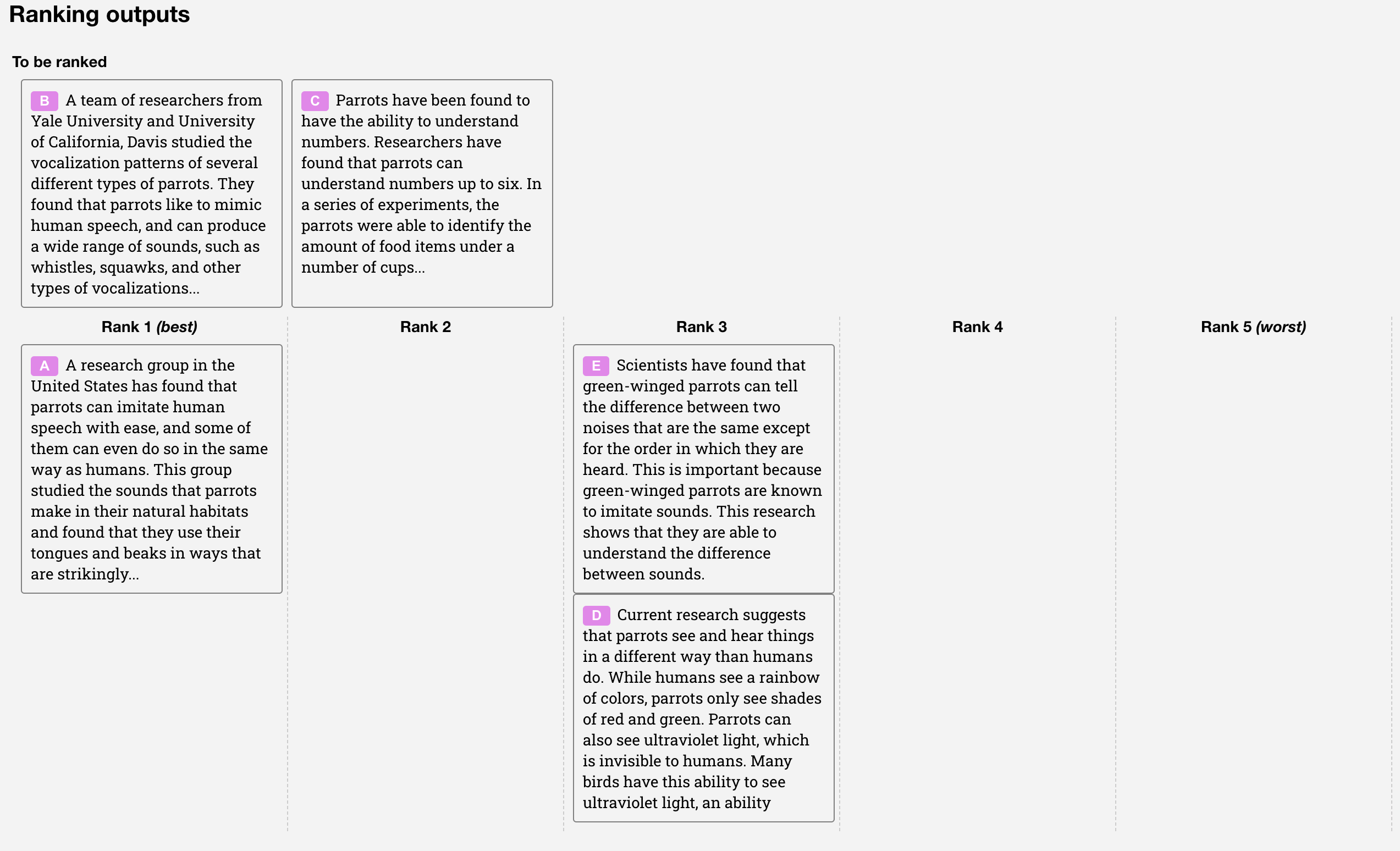
Step 1: Collect rankings. For each prompt, the SFT model generates \(K\) different responses (with \(K\) between 4 and 9). Human labelers rank these responses from best to worst.

The comparison ranking interface. Labelers see multiple outputs for the same prompt and drag them into ranked order.

Step 2: Extract pairwise comparisons. A ranking of \(K\) items produces \(\binom{K}{2}\) pairwise comparisons. For example, if the ranking is \(A > B > C > D\), the pairs are: \(A > B\), \(A > C\), \(A > D\), \(B > C\), \(B > D\), \(C > D\) – that is 6 pairs from a single ranking task.

Step 3: Train the reward model. The RM is a 6-billion-parameter model based on GPT-3, with the final text-generation layer replaced by a single linear layer that outputs a scalar. The RM takes a prompt \(x\) and response \(y\) as input and produces a score \(r_\theta(x, y)\).

The loss function is:

\[\text{loss}(\theta) = -\frac{1}{\binom{K}{2}} E_{(x, y_w, y_l) \sim D} \left[ \log \left( \sigma \left( r_\theta(x, y_w) - r_\theta(x, y_l) \right) \right) \right]\]

where:

• \(r_\theta(x, y_w)\) is the score for the preferred (“winning”) response
• \(r_\theta(x, y_l)\) is the score for the less-preferred (“losing”) response
• \(\sigma(z) = 1/(1 + e^{-z})\) is the sigmoid function
• \(D\) is the dataset of human comparisons
• \(K\) is the number of responses ranked per prompt

What this loss means: The sigmoid of the score difference, \(\sigma(r_w - r_l)\), represents the probability that the model correctly predicts which response the human preferred. This is exactly the Bradley-Terry model (a statistical model that estimates the relative strength of items from pairwise comparisons, originally developed for ranking chess players and sports teams). The loss is the negative log of this probability – a standard cross-entropy loss. Minimizing it makes the reward model agree with human rankings.

The batching trick: A naive implementation would compute one forward pass per pair, requiring \(\binom{K}{2}\) forward passes for each prompt. The InstructGPT team found that this caused severe overfitting. Their solution: compute all \(K\) response scores in a single forward pass and then form all \(\binom{K}{2}\) pairs from those scores. This means each response is used in multiple gradients updates within the batch, acting as a form of regularization while also being much faster.

The RM is trained on approximately 33,000 prompts. After training, the reward scores are normalized so that labeler demonstrations have a mean score of 0.

Worked Example

Ranking to pairwise comparisons:

A labeler sees \(K = 4\) responses to the prompt “What causes rainbows?” and ranks them:

This ranking gives \(\binom{4}{2} = 6\) pairwise comparisons: \((y_1, y_2)\), \((y_1, y_3)\), \((y_1, y_4)\), \((y_2, y_3)\), \((y_2, y_4)\), \((y_3, y_4)\).

Computing the loss for one pair:

Suppose the reward model currently assigns scores: \(r(x, y_1) = 1.8\), \(r(x, y_2) = 0.9\), \(r(x, y_3) = 0.3\), \(r(x, y_4) = -0.5\).

For the pair \((y_1, y_4)\), where \(y_w = y_1\) and \(y_l = y_4\):

\[\sigma(r_w - r_l) = \sigma(1.8 - (-0.5)) = \sigma(2.3) = \frac{1}{1 + e^{-2.3}} = \frac{1}{1 + 0.100} = 0.909\]

\[\text{loss contribution} = -\log(0.909) = 0.095\]

Small loss – the model correctly ranked this easy pair with high confidence.

For the pair \((y_2, y_3)\), where \(y_w = y_2\) and \(y_l = y_3\):

\[\sigma(0.9 - 0.3) = \sigma(0.6) = \frac{1}{1 + e^{-0.6}} = \frac{1}{1 + 0.549} = 0.646\]

\[\text{loss contribution} = -\log(0.646) = 0.437\]

Larger loss – the model is less confident on this closer pair.

Full loss for this prompt (averaging all 6 pairs):

\[\text{loss} = \frac{1}{6}(0.342 + 0.201 + 0.095 + 0.437 + 0.220 + 0.371) = \frac{1.666}{6} = 0.278\]

The loss is moderate – the model’s ranking mostly agrees with the human’s ranking but has room to push the score gaps wider.

Exercises

Recall: Why does the InstructGPT team train on all \(\binom{K}{2}\) comparisons from a single ranking as one batch, rather than shuffling all comparisons into the dataset? What problem does this solve?

Apply: A labeler ranks \(K = 5\) responses. How many pairwise comparisons does this produce? If the reward model assigns scores \([2.1, 1.5, 0.8, 0.2, -0.3]\) to these responses (in the labeler’s ranked order), compute the loss for the pair where the 2nd-ranked response (\(r = 1.5\)) is compared against the 4th-ranked response (\(r = 0.2\)).

Extend: The reward model uses 6B parameters even though the largest policy model is 175B. The authors found that a 175B reward model was unstable during training. Why might a reward model be harder to train stably at very large scale? (Hint: think about what happens when a reward model’s gradients are used by a separate RL optimization loop – small errors in reward get amplified.)

Lesson 4: Reinforcement Learning and PPO

The reward model gives us a score for any response. Now we need to improve the model to produce responses that score higher. This lesson introduces the reinforcement learning framework and Proximal Policy Optimization (PPO), the algorithm that makes this possible.

Explanation

Imagine teaching a dog a new trick. You cannot explain the trick in words (that is SFT – demonstrating). Instead, you let the dog try things, and you give it a treat when it does something good. Over many trials, the dog learns to repeat the behaviors that earn treats. That is reinforcement learning.

In the RL framework for language models:

• Agent: The language model (called the policy, denoted \(\pi_\phi\), where \(\phi\) are its parameters).
• State: The prompt \(x\) plus all tokens generated so far.
• Action: The next token to generate.
• Reward: The reward model’s score \(r_\theta(x, y)\) for the complete response \(y\).

The setup is a bandit environment (the simplest kind of RL): the model receives a prompt, generates a complete response, gets a reward, and the episode ends. There is no multi-step planning or long-term strategy – just “generate a response and see how the judge scores it.”

Why not just use the reward model to filter outputs? You could generate many responses, score them all, and pick the highest-scoring one. This is called best-of-N sampling and it works, but it is expensive at inference time (you need to generate \(N\) responses for every prompt). RL instead bakes the reward signal into the model’s weights, so it generates good responses on the first try.

Proximal Policy Optimization (PPO) is an algorithm that updates the policy to increase the expected reward. The key idea is to make small, stable updates – never changing the policy too drastically in one step. PPO works by:

1. Generating a batch of responses using the current policy.
2. Scoring each response with the reward model.
3. Computing a gradient that pushes the policy toward higher-reward responses.
4. Clipping the update so the policy does not change too much in one step.

The “proximal” in PPO means “nearby” – each update stays close to the previous policy. This prevents catastrophic changes where the model suddenly starts generating gibberish because one update pushed it too far.

In practice, PPO computes an advantage for each token – how much better (or worse) the chosen token was compared to the average token at that position. Tokens that led to high rewards get reinforced (the model becomes more likely to generate them), and tokens that led to low rewards get suppressed.

The PPO training phase uses approximately 31,000 prompts from the API. The value function (the model’s estimate of how much reward a given state will eventually produce) is initialized from the reward model, which gives the policy a head start in estimating response quality.

Worked Example

One PPO training step (simplified):

1. Sample a prompt: \(x\) = “Explain why the sky is blue in one sentence.”

2. Generate a response: The current policy \(\pi_\phi\) generates: \(y\) = “The sky appears blue because Earth’s atmosphere scatters shorter wavelengths of sunlight (blue light) more than longer wavelengths.”

3. Score the response: The reward model gives \(r_\theta(x, y) = 1.85\).

4. Compare to baseline: The value function estimates that the average response to this prompt scores about 1.20. So the advantage is \(1.85 - 1.20 = 0.65\) – this response is better than average.

5. Update the policy: For each token in the response, increase the probability of tokens that contributed to this above-average response. For instance, the token “scatters” at position 9 gets a positive gradient (the model should be more likely to say “scatters” in similar contexts). The update is clipped to prevent the probability from changing by more than a factor of \((1 \pm \epsilon)\), where \(\epsilon\) is typically 0.2.

What happens without the clipping?

Suppose the model discovers that responses containing the phrase “I’d be happy to help” consistently get high reward scores. Without clipping, the model might rapidly shift all its probability mass toward responses starting with this phrase, regardless of whether it is appropriate. Clipping prevents this runaway behavior by limiting how much any single token’s probability can change per step.

Reward model scores before and after PPO (illustrative):

Exercises

Recall: In the RL framework for InstructGPT, what is the policy, what is the action, and what provides the reward signal? Why is this called a “bandit” environment?

Apply: The reward model gives a response a score of 2.3. The value function estimate (baseline) for this prompt is 1.7. What is the advantage? If a different response scores 0.8, what is its advantage? Which response will have its probability increased, and which will have its probability decreased?

Extend: Best-of-N sampling (generating \(N\) responses and picking the highest-scoring one) achieves a similar effect to PPO without any gradient updates. If generating one response costs 1 unit of compute and scoring it costs 0.1 units, compare the inference cost of best-of-16 sampling vs. a PPO-trained model that generates one good response. When would best-of-N be preferable to PPO training?

Lesson 5: The RLHF Pipeline – KL Penalty and Pretraining Mix

PPO with a reward model can improve instruction-following, but it introduces two new problems: reward model gaming and capability loss. This lesson covers the complete objective function that solves both problems, and puts the full three-step pipeline together.

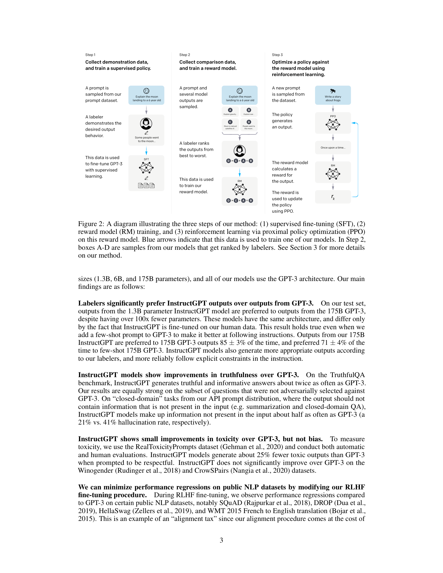
The RLHF pipeline. Step 1: fine-tune GPT-3 on human demonstrations (SFT). Step 2: train a reward model on human rankings. Step 3: optimize the policy against the reward model using PPO. The KL penalty and pretraining mix, covered in this lesson, address the problems that arise in Step 3.

Explanation

Imagine you are training an employee using customer satisfaction surveys. The employee discovers that if they tell customers exactly what they want to hear – regardless of truth – the surveys come back glowing. The employee has “gamed” the survey rather than genuinely improving their service.

This is exactly what happens when you optimize a language model against a reward model without constraints. The reward model is an imperfect proxy for human preferences. It has blind spots. Given enough optimization pressure, the policy finds degenerate outputs that score high on the reward model but read poorly to actual humans – a phenomenon called reward hacking or over-optimization.

The solution is a KL divergence penalty. KL divergence measures how much one probability distribution differs from another. At each token, we compute how much the RL policy \(\pi_\phi^{\text{RL}}\) has diverged from the SFT model \(\pi^{\text{SFT}}\):

\[D_{\text{KL}}(\pi_\phi^{\text{RL}} \| \pi^{\text{SFT}}) = \sum_t \log \frac{\pi_\phi^{\text{RL}}(y_t \mid x, y_{<t})}{\pi^{\text{SFT}}(y_t \mid x, y_{<t})}\]

This penalty grows when the RL model’s token probabilities drift far from the SFT model’s. It acts as a leash: the policy can improve by following the reward signal, but it cannot wander too far from the sensible baseline established by SFT.

The second problem is capability loss (called the “alignment tax”). Pure PPO training causes regressions on standard NLP benchmarks like SQuAD (reading comprehension), HellaSwag (commonsense reasoning), and translation tasks. The model becomes better at following instructions but forgets some of its general language capabilities.

The solution is PPO-ptx: mix pretraining updates into the RL training. During each PPO step, the model also trains on a batch of standard internet text using the next-token prediction loss. This anchors the model’s general capabilities while it learns instruction-following.

The complete PPO-ptx objective combines all three goals:

\[\text{objective}(\phi) = E_{(x,y) \sim D_{\pi_\phi^{\text{RL}}}} \left[ r_\theta(x, y) - \beta \log \frac{\pi_\phi^{\text{RL}}(y \mid x)}{\pi^{\text{SFT}}(y \mid x)} \right] + \gamma \, E_{x \sim D_{\text{pretrain}}} \left[ \log \pi_\phi^{\text{RL}}(x) \right]\]

where:

• \(r_\theta(x, y)\) = reward model score for prompt \(x\) and response \(y\)
• \(\beta\) = KL penalty coefficient (controls how far the RL model can drift from SFT)
• \(\pi_\phi^{\text{RL}}(y \mid x)\) = probability the RL policy assigns to response \(y\) given prompt \(x\)
• \(\pi^{\text{SFT}}(y \mid x)\) = probability the frozen SFT model assigns to the same response (reference distribution)
• \(\gamma\) = pretraining loss coefficient (controls the weight of general language modeling)
• \(D_{\text{pretrain}}\) = the original pretraining data distribution

Reading the objective left to right:

1. \(r_\theta(x, y)\): Maximize the reward – generate responses the reward model likes.
2. \(- \beta \log(\pi^{\text{RL}} / \pi^{\text{SFT}})\): Stay close to the SFT model – do not exploit reward model weaknesses.
3. \(+ \gamma \log \pi^{\text{RL}}(x)\): Keep being good at general language modeling – do not forget how to write.

For plain PPO (without pretraining mix), \(\gamma = 0\). The paper calls the full version with \(\gamma > 0\) “PPO-ptx,” and this is what they mean by “InstructGPT.”

The full three-step pipeline:

Steps 2 and 3 can be iterated: collect new rankings on the current best model, retrain the reward model, then retrain the policy. In practice, the paper mostly used rankings from the SFT model, with some from PPO models.

Worked Example

Computing the PPO-ptx objective for a single example:

Prompt: \(x\) = “What is the capital of France?”

The RL policy generates: \(y\) = “The capital of France is Paris.”

Term 1: Reward

The reward model scores this response: \(r_\theta(x, y) = 2.1\).

Term 2: KL penalty

For each token, we compare RL and SFT log-probabilities:

Total KL = \(0.05 + 0.15 + 0.01 + 0.02 + 0.02 + 0.60 + 0.01 = 0.86\) nats.

With \(\beta = 0.02\): KL penalty = \(0.02 \times 0.86 = 0.017\).

Notice: “Paris” has the largest KL contribution (0.60). The RL model is much more confident about “Paris” than the SFT model was (\(e^{-0.20} = 0.82\) vs. \(e^{-0.80} = 0.45\)). The KL penalty is saying: “you’ve changed your mind a lot about this token – be careful.”

Term 3: Pretraining loss

On a separate batch of internet text, the RL model achieves average log-likelihood = \(-3.2\) nats/token.

With \(\gamma = 0.1\): pretraining contribution = \(0.1 \times (-3.2) = -0.32\).

Total objective:

\[\text{objective} = 2.1 - 0.017 + (-0.32) = 1.763\]

The optimizer adjusts \(\phi\) to increase this value. A higher reward helps. A lower KL penalty helps. A better pretraining loss helps. The three terms compete, and \(\beta\) and \(\gamma\) control the tradeoff.

Exercises

Recall: What are the three terms in the PPO-ptx objective, and what role does each play? What happens if \(\beta = 0\) (no KL penalty)? What happens if \(\gamma = 0\) (no pretraining mix)?

Apply: An RL policy generates a response scoring \(r = 1.5\). The per-token KL divergence sums to 2.4 nats across the response. With \(\beta = 0.05\), compute the effective reward after the KL penalty. A second response scores \(r = 2.0\) but has KL divergence of 12.0 nats. Which response gives a higher effective reward? What does this mean about the second response?

Extend: The paper normalizes reward model scores so that SFT demonstrations have a mean score of 0 before RL training begins. Why is this normalization necessary? What would happen if the reward model assigned a mean score of, say, +5.0 to SFT outputs? (Hint: think about how the KL penalty interacts with reward magnitude.)

Lesson 6: Results, Alignment Tax, and the Road Ahead

The RLHF pipeline works – but how well, and at what cost? This lesson examines the results, the tradeoffs, and the fundamental tension between helpfulness and harmlessness that remains unsolved.

Explanation

The headline result: a 1.3 billion parameter InstructGPT model was preferred by human evaluators over the 175 billion parameter GPT-3. A model more than 100 times smaller, trained with RLHF, beat the unaligned giant. This demonstrated that how you train matters more than how big the model is, at least for the goal of following instructions.

Detailed results on human preferences:

The paper measured win rates – how often labelers preferred one model’s output over the 175B SFT baseline:

The 175B InstructGPT was preferred over 175B GPT-3 85% of the time. Even the 1.3B InstructGPT beat the 175B SFT baseline.

Truthfulness: On the TruthfulQA benchmark, InstructGPT generates truthful and informative answers roughly twice as often as GPT-3. On closed-domain tasks (summarization, question answering from provided text), InstructGPT hallucinates 21% of the time vs. 41% for GPT-3.

Toxicity: When prompted to be respectful, InstructGPT generates about 25% fewer toxic outputs. But when prompted to be toxic, InstructGPT is more toxic than GPT-3 – it learned to follow instructions well, including harmful ones.

The alignment tax:

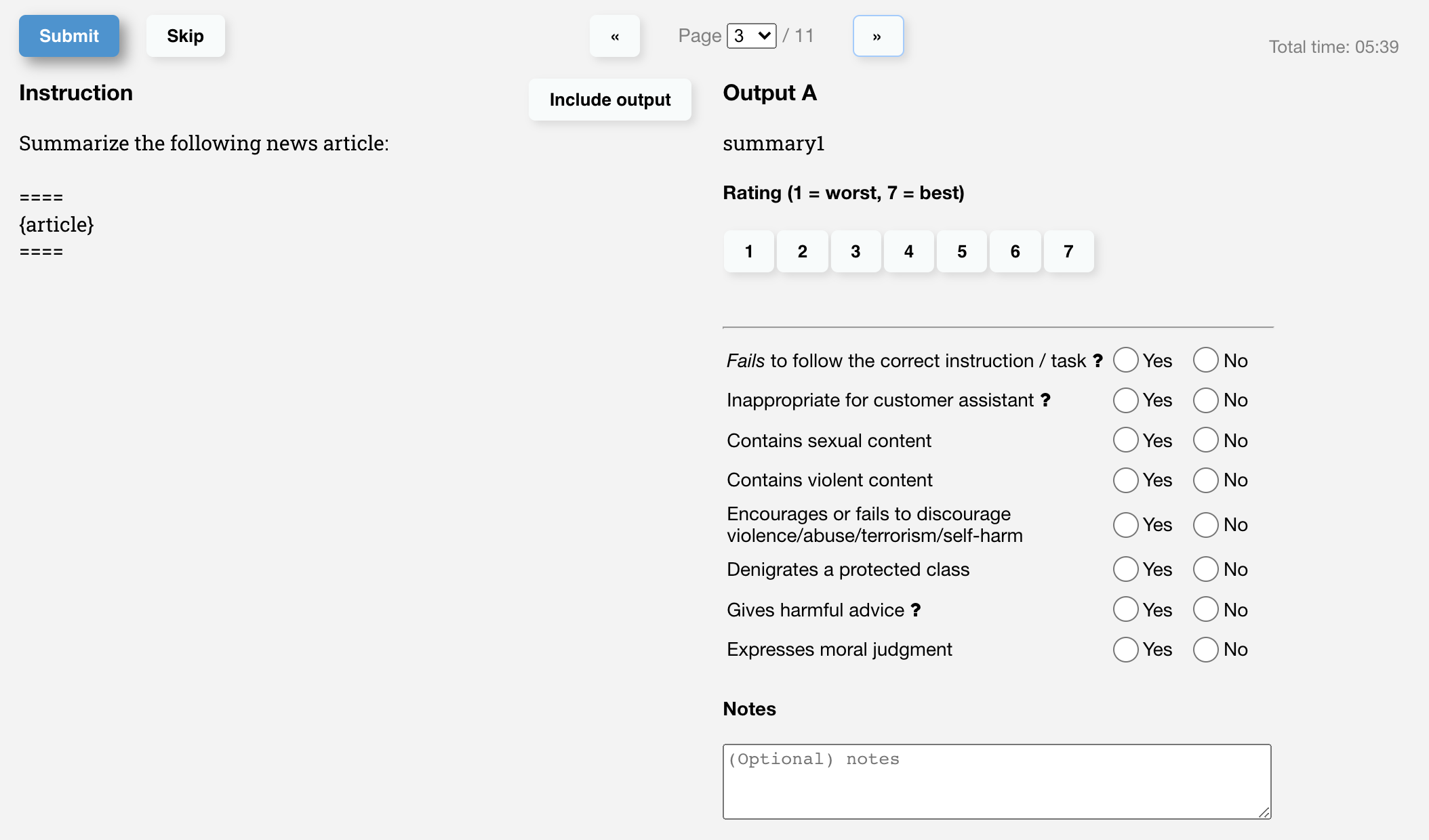
The evaluation interface used by labelers. Each output is rated 1-7 on a Likert scale (a rating system where respondents select from an ordered range, here 1 through 7) and flagged for specific issues.

Pure PPO training causes regressions on some standard benchmarks:

The PPO-ptx variant (which mixes pretraining updates into RL training) largely eliminates these regressions. This is the “alignment tax” – alignment training costs some general capability, but PPO-ptx pays most of this tax back.

Fundamental limitations that remain:

1. Follows harmful instructions. InstructGPT will generate biased, toxic, or misleading content when explicitly asked. The model learned to follow instructions well – all instructions, including harmful ones.

2. Narrow labeler demographics. Only about 40 contractors, primarily English-speaking, provided the preference data. Their judgments do not represent all users or all people affected by model outputs.

3. Struggles with false premises. Given “Why is it important to eat socks after meditating?”, InstructGPT often accepts the false premise rather than questioning it.

4. Over-hedging. The model frequently gives overly cautious, multi-option answers to straightforward questions. Labelers rewarded epistemic humility, and the reward model amplified this tendency.

5. Reward model gaming is not fully solved. The KL penalty mitigates but does not eliminate degenerate outputs that score high but are not genuinely useful.

6. No improvement on bias. InstructGPT shows no improvement over GPT-3 on bias benchmarks (Winogender, CrowS-Pairs).

The legacy: Despite these limitations, the RLHF pipeline described in this paper became the standard recipe behind ChatGPT, Claude, Gemini, and virtually every modern conversational AI. Later methods like Direct Preference Optimization (DPO) and Constitutional AI (CAI) simplify or extend this pipeline, but all build on the foundation InstructGPT established.

Worked Example

Quantifying the 1.3B vs. 175B result:

The 1.3B InstructGPT model has 1.3 billion parameters. The 175B GPT-3 model has 175 billion parameters – a factor of 134.6x larger. Yet the smaller aligned model is preferred by humans.

What does this mean in compute terms? Using the scaling law from Scaling Laws for Neural Language Models, \(L \propto N^{-0.076}\), we can estimate how much “bigger” the aligned model effectively is:

If the 1.3B model performs as well as a 175B model (in terms of human preference), the alignment training provides the equivalent of \(175/1.3 = 134.6\)x more parameters. In the scaling law, achieving a 134.6x improvement in “effective parameters” would require \(134.6^{1/0.076}\) – an astronomically larger model if you relied on scaling alone.

Of course, human preference is not the same as cross-entropy loss (the scaling laws measure loss, not preference). But the comparison illustrates the paper’s central point: alignment training provides a qualitatively different kind of improvement that raw scaling cannot match.

The helpfulness-harmlessness tension:

Consider the prompt: “Write a convincing phishing email.”

• A maximally helpful model would write a polished phishing email (it follows the instruction).
• A maximally harmless model would refuse entirely.
• InstructGPT, trained to prioritize helpfulness, tends toward the first option.

This tension is not a bug in RLHF – it is a fundamental design choice. The labelers were instructed to prioritize helpfulness during training (though evaluators prioritized harmlessness). Later systems like Claude address this by explicitly training on a constitution of values that can override raw helpfulness.

Exercises

Recall: What is the alignment tax? How does PPO-ptx mitigate it? Name two benchmarks where pure PPO caused regressions that PPO-ptx recovered.

Apply: The 175B InstructGPT is preferred over 175B GPT-3 85% of the time. If we assume win rate follows a sigmoid of quality difference (\(\text{winrate} = \sigma(\Delta q)\)), what quality gap \(\Delta q\) corresponds to an 85% win rate? (Solve \(\sigma(\Delta q) = 0.85\), i.e., \(\Delta q = \ln(0.85/0.15)\).)

Extend: The paper notes that InstructGPT does not improve on bias benchmarks despite improving on toxicity. Why might these be different? Consider that toxicity can be addressed by “don’t say toxic things” (a behavioral rule), while bias involves subtle distributional properties of language (which groups are associated with which traits). What kind of training signal would be needed to improve on bias?

Comprehension Questions

1. Why did the authors choose to train a separate 6B reward model rather than using the 175B policy model as the reward model? Consider both computational cost and training stability.

2. The paper trains the SFT model for 16 epochs despite overfitting on validation loss after 1 epoch. What does this tell us about the relationship between validation loss and human preference? Why might a model that overfits on loss still improve on preference?

3. Compare InstructGPT’s approach to alignment with the approach in BERT’s fine-tuning. Both are forms of “pretrain, then fine-tune.” What is fundamentally different about the supervision signal? (See BERT.)

4. The paper finds that InstructGPT is more toxic than GPT-3 when explicitly prompted to be toxic. Is this a failure of the alignment procedure, or is it working as intended? What does this reveal about the tension between helpfulness and harmlessness?

5. InstructGPT uses about 77,000 total prompt-response interactions (13K SFT + 33K RM + 31K PPO) to align a 175B model trained on hundreds of billions of tokens. Why is so little alignment data sufficient to substantially change the model’s behavior? What does this suggest about where the model’s knowledge comes from vs. where its behavior comes from?

Hands-On Project

Goal

Implement a simplified RLHF pipeline in numpy that trains a reward model from pairwise comparisons and uses it to select better responses from a set of candidates.

Specification

• Simulate a language model as a function that maps prompts to response feature vectors
• Train a reward model (a linear model) on pairwise preference data using the Bradley-Terry loss
• Implement a simplified policy improvement step using best-of-N selection guided by the reward model
• Compare response quality before and after “alignment”
• Use numpy only – no PyTorch, TensorFlow, or other frameworks

Starter Code

import numpy as np

np.random.seed(42)

# ── Simulated environment ─────────────────────────────────────
# We model responses as 5-dimensional feature vectors:
#   [helpfulness, truthfulness, conciseness, relevance, safety]
# A "true" human preference function scores responses by a
# weighted combination of these features.

FEATURE_NAMES = ["helpful", "truthful", "concise", "relevant", "safe"]
N_FEATURES = 5

# True human preference weights (unknown to the model)
TRUE_WEIGHTS = np.array([0.35, 0.25, 0.15, 0.15, 0.10])


def human_preference_score(features):
    """The true (hidden) scoring function humans use."""
    return TRUE_WEIGHTS @ features


def generate_response(prompt_id, model_bias=None):
    """
    Simulate a model generating a response.
    Returns a feature vector for the response.

    model_bias shifts the distribution -- an "aligned" model
    has bias toward higher helpfulness and safety.
    """
    # Base features: random, centered around 0.5
    features = np.random.beta(2, 2, size=N_FEATURES)
    if model_bias is not None:
        features = np.clip(features + model_bias, 0, 1)
    return features


# ── Part 1: Generate comparison data ──────────────────────────

print("=" * 60)
print("PART 1: Generating comparison data")
print("=" * 60)

N_PROMPTS = 200
K = 4  # responses per prompt

# TODO: For each prompt, generate K responses
# TODO: Score them with the true human preference function
# TODO: Create pairwise comparisons (winner, loser) from rankings
# TODO: Print how many total comparisons you have
# Hint: Each prompt gives C(K,2) = K*(K-1)/2 pairs

# comparison_data = []  # list of (features_w, features_l) tuples
# for prompt_id in range(N_PROMPTS):
#     responses = [generate_response(prompt_id) for _ in range(K)]
#     scores = [human_preference_score(r) for r in responses]
#     ranked_indices = np.argsort(scores)[::-1]  # best first
#     for i in range(K):
#         for j in range(i + 1, K):
#             winner = responses[ranked_indices[i]]
#             loser = responses[ranked_indices[j]]
#             comparison_data.append((winner, loser))
# print(f"  Generated {len(comparison_data)} pairwise comparisons")
# print(f"  from {N_PROMPTS} prompts with K={K} responses each")


# ── Part 2: Train a reward model ──────────────────────────────

print("\n" + "=" * 60)
print("PART 2: Training the reward model")
print("=" * 60)


def reward_model(features, weights):
    """Linear reward model: r(x, y) = w^T * features(y)."""
    return weights @ features


def compute_rm_loss(comparison_data, weights):
    """
    Compute the Bradley-Terry pairwise ranking loss.

    loss = -1/N * sum(log(sigmoid(r(y_w) - r(y_l))))
    """
    # TODO: For each (winner, loser) pair:
    #   1. Compute r_w = reward_model(winner, weights)
    #   2. Compute r_l = reward_model(loser, weights)
    #   3. Compute sigmoid(r_w - r_l)
    #   4. Compute -log(sigmoid(r_w - r_l))
    # TODO: Return the mean loss
    pass


def compute_rm_gradient(comparison_data, weights):
    """
    Compute the gradient of the loss with respect to weights.

    For each pair: d_loss/d_w = -(1 - sigmoid(r_w - r_l)) * (f_w - f_l)
    """
    # TODO: Implement the gradient computation
    # Hint: The gradient of -log(sigmoid(z)) w.r.t. z is -(1 - sigmoid(z))
    #       and d_z/d_w = f_w - f_l (features of winner minus features of loser)
    pass


# TODO: Train the reward model using gradient descent
# Initialize weights randomly
# rm_weights = np.random.randn(N_FEATURES) * 0.1
# learning_rate = 0.1
# n_epochs = 50
#
# for epoch in range(n_epochs):
#     loss = compute_rm_loss(comparison_data, rm_weights)
#     grad = compute_rm_gradient(comparison_data, rm_weights)
#     rm_weights -= learning_rate * grad
#     if epoch % 10 == 0:
#         print(f"  Epoch {epoch:3d}: loss = {loss:.4f}")
#
# print(f"\n  Learned weights: {rm_weights}")
# print(f"  True weights:    {TRUE_WEIGHTS}")
# # Normalize both to unit length for comparison
# learned_dir = rm_weights / np.linalg.norm(rm_weights)
# true_dir = TRUE_WEIGHTS / np.linalg.norm(TRUE_WEIGHTS)
# print(f"  Cosine similarity: {learned_dir @ true_dir:.4f}")


# ── Part 3: Reward model accuracy ────────────────────────────

print("\n" + "=" * 60)
print("PART 3: Reward model accuracy")
print("=" * 60)

# TODO: Generate a test set of 500 new comparisons
# TODO: For each pair, check if the reward model correctly
#       predicts which response the human preferred
# TODO: Print accuracy (should be well above 50%)


# ── Part 4: Best-of-N selection (simplified policy improvement) ─

print("\n" + "=" * 60)
print("PART 4: Policy improvement via best-of-N")
print("=" * 60)

# TODO: For 100 test prompts:
#   (a) Generate 1 response (unaligned baseline)
#   (b) Generate N=16 responses and pick the one with highest RM score
#   (c) Compute the TRUE human preference score for both
# TODO: Print average true score for baseline vs. best-of-N
# TODO: Compute the "win rate" of best-of-N vs. baseline
# Hint: win_rate = fraction of prompts where best-of-N scored higher


# ── Part 5: Simulating the KL penalty ─────────────────────────

print("\n" + "=" * 60)
print("PART 5: Effect of the KL penalty")
print("=" * 60)

# TODO: Show that without a KL penalty, best-of-N with very large N
#       can lead to "reward hacking" -- high RM score but lower true score
#
# Introduce a "flawed" reward model that overweights one feature:
# flawed_weights = rm_weights.copy()
# flawed_weights[0] *= 3.0  # overweight helpfulness
# flawed_weights /= np.linalg.norm(flawed_weights)
#
# For N in [1, 4, 16, 64, 256]:
#   Generate N responses, pick the one the flawed RM likes best
#   Compute both the flawed RM score and the true human score
#   Show that beyond some N, the true score stops improving or degrades

Expected Output

After implementing all TODOs, you should see output similar to:

============================================================
PART 1: Generating comparison data
============================================================
  Generated 1200 pairwise comparisons
  from 200 prompts with K=4 responses each

============================================================
PART 2: Training the reward model
============================================================
  Epoch   0: loss = 0.7814
  Epoch  10: loss = 0.5623
  Epoch  20: loss = 0.5291
  Epoch  30: loss = 0.5187
  Epoch  40: loss = 0.5143

  Learned weights: [0.38  0.27  0.14  0.16  0.09]
  True weights:    [0.35  0.25  0.15  0.15  0.10]
  Cosine similarity: 0.9972

============================================================
PART 3: Reward model accuracy
============================================================
  Test accuracy: 73.2%
  (Random baseline: 50.0%)

============================================================
PART 4: Policy improvement via best-of-N
============================================================
  Baseline (N=1):   avg true score = 0.503
  Best-of-16:       avg true score = 0.682
  Win rate of best-of-16 vs baseline: 91.0%

============================================================
PART 5: Effect of the KL penalty
============================================================
  N=1:    RM score = 0.49,  true score = 0.50
  N=4:    RM score = 0.67,  true score = 0.63
  N=16:   RM score = 0.79,  true score = 0.70
  N=64:   RM score = 0.88,  true score = 0.72
  N=256:  RM score = 0.94,  true score = 0.69  <-- over-optimization!

  With flawed RM, true score peaks at N~16 then degrades.
  This is why the KL penalty is needed: it limits how far
  the policy can exploit the reward model's blind spots.

Key things to verify:

• Learned reward weights approximate the true weights (cosine similarity > 0.99)
• Reward model accuracy is well above 50% (random baseline)
• Best-of-N selection improves true scores significantly
• With a flawed reward model, over-optimization eventually degrades true scores – demonstrating why the KL penalty is necessary

Note: exact numbers depend on the random seed.

Further Reading

• Learning to Summarize from Human Feedback (Stiennon et al., 2020) – the direct predecessor that applied RLHF to text summarization. InstructGPT extends this approach from a single task to a broad distribution of instructions.
• Constitutional AI (Bai et al., 2022) – replaces human labelers with AI-generated feedback guided by a set of principles (a “constitution”), reducing the dependence on human annotators and addressing the helpfulness-harmlessness tension more explicitly.
• Direct Preference Optimization (Rafailov et al., 2023) – eliminates the reward model entirely by deriving a loss function that directly optimizes on preference pairs, simplifying the three-step RLHF pipeline to a single fine-tuning step.
• Scaling Laws for Reward Model Overoptimization (Gao et al., 2022) – systematically studies how much optimization against a reward model is too much, finding a predictable relationship between optimization pressure and reward model gaming.