LoRA: Low-Rank Adaptation of Large Language Models: Course

Learning Objectives

By the end of this course, you will be able to:

1. Explain why full fine-tuning and adapter methods both fall short for deploying many task-specific versions of a large model
2. Decompose a matrix into the product of two smaller matrices and calculate the parameter savings of a rank-\(r\) factorization
3. Compute the LoRA forward pass by hand, including the low-rank branch and scaling factor
4. Describe LoRA’s initialization scheme and explain why starting from zero change is critical
5. Determine which weight matrices to adapt and calculate the total trainable parameter count for a given configuration
6. Merge LoRA weights into the base model and perform task switching without reloading the full model

Prerequisites

• Python and numpy – comfortable with functions, array operations, and matrix multiplication
• Matrix multiplication – multiplying an \((n \times m)\) matrix by an \((m \times p)\) matrix to produce an \((n \times p)\) result (see Attention Is All You Need course for a refresher)
• The Transformer architecture – multi-head self-attention with query, key, value, and output projections (see Attention Is All You Need course)
• Pre-training and fine-tuning – the two-phase paradigm where a model first learns general language patterns, then specializes on a task (see GPT course)
• Adapter-based transfer learning – inserting small trainable bottleneck modules into a frozen model (see Parameter-Efficient Transfer Learning course)

Lesson 1: Why Adapters Are Not Enough

Lesson 5 of the adapter course (see Parameter-Efficient Transfer Learning) showed that inserting small bottleneck modules into a frozen Transformer can reduce trainable parameters from 100% to about 2-4% per task with minimal accuracy loss. Problem solved? Not quite. Adapters fix the storage problem but introduce a new one: inference latency.

Explanation

Recall the adapter architecture: each adapter module sits inside the Transformer layer as a sequential bottleneck – data flows through the frozen sub-layer, then through the adapter, then onward. The adapter is an extra computation step that every token must pass through at every layer, during both training and inference. When the model is small and the batch is large, this overhead is negligible because the GPU has enough parallel work to hide it. But when the batch size is small – as it typically is in real-time applications like chatbots – the adapter latency becomes significant.

The LoRA paper measured this directly on GPT-2 medium (345M parameters) with a single NVIDIA RTX8000 GPU:

At batch size 1 (the common case for interactive serving), the Houlsby adapter adds 30% latency. This is because adapters are sequential – data must flow through them one after another, and no amount of hardware parallelism helps when the operations are on the critical path.

The other existing approach, prefix tuning, prepends learnable tokens to the input. But those tokens consume part of the limited sequence length, leaving less room for the actual task input. And prefix tuning is difficult to optimize – performance changes non-monotonically (it does not consistently improve or degrade, but fluctuates unpredictably) as you add more prefix tokens.

The field needs a method that achieves three things simultaneously:

1. Parameter efficiency – train and store a tiny fraction of the full model
2. No inference latency – the adapted model runs at exactly the same speed as the original
3. Quality parity – match or beat full fine-tuning accuracy

LoRA delivers all three. The key idea: instead of adding new layers in series (adapters) or prepending tokens (prefix tuning), LoRA modifies the existing weight matrices in parallel through a low-rank update that can be absorbed into the original weights at deployment time.

Worked Example

Suppose you deploy GPT-3 (175B parameters) for 100 customers, each with a different fine-tuned version. Compare the storage costs:

Full fine-tuning: each customer gets a separate copy of all 175B parameters stored in 16-bit floating point (2 bytes per parameter).

• Per-customer: \(175 \times 10^9 \times 2 = 350\) GB
• Total: \(100 \times 350 = 35{,}000\) GB = 35 TB

Adapter tuning: one shared base model plus adapters per customer. Adapters at 0.04% of parameters (\({\approx}7.1\)M) reduce per-task storage, but every forward pass still runs through adapter layers.

• Shared: 350 GB
• Per-customer adapters: \(7.1 \times 10^6 \times 2 \approx 14\) MB
• Total: \(350 + 100 \times 0.014 = 351.4\) GB (storage is good, but 20-30% slower inference)

LoRA (\(r = 4\), adapting \(W_q\) and \(W_v\)): one shared base model plus tiny LoRA matrices per customer, merged into the base weights at serving time.

• Shared: 350 GB
• Per-customer LoRA: \(4.7 \times 10^6 \times 2 \approx 9.4\) MB
• Total: \(350 + 100 \times 0.0094 \approx 350.9\) GB (storage is good and inference is identical to the original model)

Exercises

Recall: What are the two practical problems with adapter layers that LoRA aims to solve? Why does batch size affect the severity of the adapter latency problem?

Apply: A company runs GPT-2 medium (345M parameters) with Adapter\(^H\) at batch size 1, serving 500 requests per second. Each request takes 25.8 ms with adapters versus 19.8 ms without. How many more GPU-seconds per hour does the adapter overhead cost? How many additional GPUs (at 100% utilization) would be needed to maintain the same throughput?

Extend: Prefix tuning and LoRA both avoid adding sequential layers, yet the LoRA paper shows prefix tuning performs worse as you increase parameters. The paper hypothesizes this is because extra prefix tokens shift the input distribution away from what the model saw during pre-training. Can you think of a task where this distribution shift would be especially harmful? What about one where it might matter less?

Lesson 2: Matrix Rank and Low-Rank Factorization

Think of a 1000-page cookbook that uses only 5 fundamental sauces. Every recipe is a variation on those 5 bases. You could describe the entire book as “here are 5 base sauces” plus “here is how each recipe tweaks the base.” The book has 1000 rows (recipes) and many columns (ingredients), but its true dimensionality is only 5 – the number of independent sauce bases. That number is the rank.

Explanation

The rank of a matrix is the number of linearly independent rows (or equivalently, columns) it contains. A matrix \(M \in \mathbb{R}^{d \times k}\) has at most \(\min(d, k)\) independent rows or columns, so \(\text{rank}(M) \leq \min(d, k)\). When a matrix has rank \(r\) much smaller than its dimensions, we say it is low-rank or rank-deficient.

The critical property of a rank-\(r\) matrix is that it can always be written as the product of two smaller matrices:

\[M = B A\]

where \(B \in \mathbb{R}^{d \times r}\) and \(A \in \mathbb{R}^{r \times k}\). This is called a low-rank factorization. The matrix \(M\) has \(d \times k\) entries, but storing \(B\) and \(A\) requires only \(d \times r + r \times k\) entries – a huge savings when \(r \ll \min(d, k)\).

The parameter savings ratio is:

\[\text{compression ratio} = \frac{d \times k}{d \times r + r \times k} = \frac{dk}{r(d + k)}\]

For square matrices where \(d = k\):

\[\text{compression ratio} = \frac{d^2}{2dr} = \frac{d}{2r}\]

This ratio grows linearly with the matrix dimension. For a \(12{,}288 \times 12{,}288\) weight matrix in GPT-3 with rank \(r = 4\), the compression ratio is \(\frac{12{,}288}{2 \times 4} = 1{,}536\). Instead of storing 150 million numbers, you store about 98 thousand.

Why would the change needed to adapt a model be low-rank? Prior work by Aghajanyan et al. (2020) showed that large pre-trained models have a low “intrinsic dimensionality” – despite having billions of parameters, they effectively operate in a much smaller subspace. LoRA extends this idea: if the model itself lives in a low-dimensional space, then the update needed to shift it from general behavior to task-specific behavior might also be low-dimensional. Instead of allowing the update \(\Delta W\) to be any arbitrary matrix, LoRA forces it to have rank at most \(r\) by constructing it as the product \(BA\).

Worked Example

Let \(d = 4\), \(k = 4\), and \(r = 2\). We want to represent a \(4 \times 4\) update matrix as the product of a \(4 \times 2\) matrix and a \(2 \times 4\) matrix.

\[B = \begin{bmatrix} 0.1 & 0.3 \\ 0.2 & -0.1 \\ -0.3 & 0.2 \\ 0.4 & 0.1 \end{bmatrix}, \quad A = \begin{bmatrix} 0.5 & -0.2 & 0.1 & 0.3 \\ -0.1 & 0.4 & 0.2 & -0.3 \end{bmatrix}\]

Their product \(\Delta W = BA\) is:

\[\Delta W = \begin{bmatrix} (0.1)(0.5) + (0.3)(-0.1) & (0.1)(-0.2) + (0.3)(0.4) & (0.1)(0.1) + (0.3)(0.2) & (0.1)(0.3) + (0.3)(-0.3) \\ (0.2)(0.5) + (-0.1)(-0.1) & (0.2)(-0.2) + (-0.1)(0.4) & (0.2)(0.1) + (-0.1)(0.2) & (0.2)(0.3) + (-0.1)(-0.3) \\ (-0.3)(0.5) + (0.2)(-0.1) & (-0.3)(-0.2) + (0.2)(0.4) & (-0.3)(0.1) + (0.2)(0.2) & (-0.3)(0.3) + (0.2)(-0.3) \\ (0.4)(0.5) + (0.1)(-0.1) & (0.4)(-0.2) + (0.1)(0.4) & (0.4)(0.1) + (0.1)(0.2) & (0.4)(0.3) + (0.1)(-0.3) \end{bmatrix}\]

\[= \begin{bmatrix} 0.02 & 0.10 & 0.07 & 0.00 \\ 0.11 & -0.08 & 0.00 & 0.09 \\ -0.17 & 0.14 & 0.01 & -0.15 \\ 0.19 & -0.04 & 0.06 & 0.09 \end{bmatrix}\]

\(\Delta W\) is a \(4 \times 4\) matrix with 16 entries, but we only stored \(B\) (8 entries) and \(A\) (8 entries) = 16 total. At this tiny scale, there is no savings. But now scale up:

• GPT-3 scale: \(d = k = 12{,}288\), \(r = 4\). Original: \(12{,}288^2 = 150{,}994{,}944\) entries. Factored: \(12{,}288 \times 4 + 4 \times 12{,}288 = 98{,}304\) entries. Compression: \(1{,}536\times\).

The rank-\(r\) factorization constrains \(\Delta W\) to a \(r\)-dimensional subspace. Every column of \(\Delta W\) is a linear combination of the \(r\) columns of \(B\), and every row is a linear combination of the \(r\) rows of \(A\). This is a strong constraint – but if the task-adaptation signal really is low-rank, it is exactly the right constraint.

Exercises

Recall: If a matrix \(M \in \mathbb{R}^{100 \times 200}\) has rank 3, what are the dimensions of the two matrices in its low-rank factorization? How many total entries do they contain, compared to the original?

Apply: A Transformer has \(d_{\text{model}} = 768\) (BERT-Base scale). A weight matrix \(W_q\) is \(768 \times 768\). Calculate the number of parameters for: (a) the full matrix, (b) a rank-4 factorization, (c) a rank-1 factorization. Express each factored count as a percentage of the full matrix.

Extend: Not every matrix is low-rank. If you forced a rank-2 factorization on a full-rank \(100 \times 100\) matrix, you would lose information. In what sense does LoRA bet that this information loss is acceptable? Under what conditions might this bet fail? (Hint: think about adapting a model to a language it was never pre-trained on.)

Lesson 3: The LoRA Forward Pass

Imagine you have a professional camera with a fixed lens (the pre-trained weight matrix). Instead of replacing the entire lens for a different style of photography (full fine-tuning), you snap on a thin filter (the low-rank matrices \(B\) and \(A\)). The filter adjusts the image subtly – it does not change the lens, and the light still passes through both in parallel. When you are done, you can bake the filter effect directly into a new lens (merge), and nobody can tell a filter was ever used.

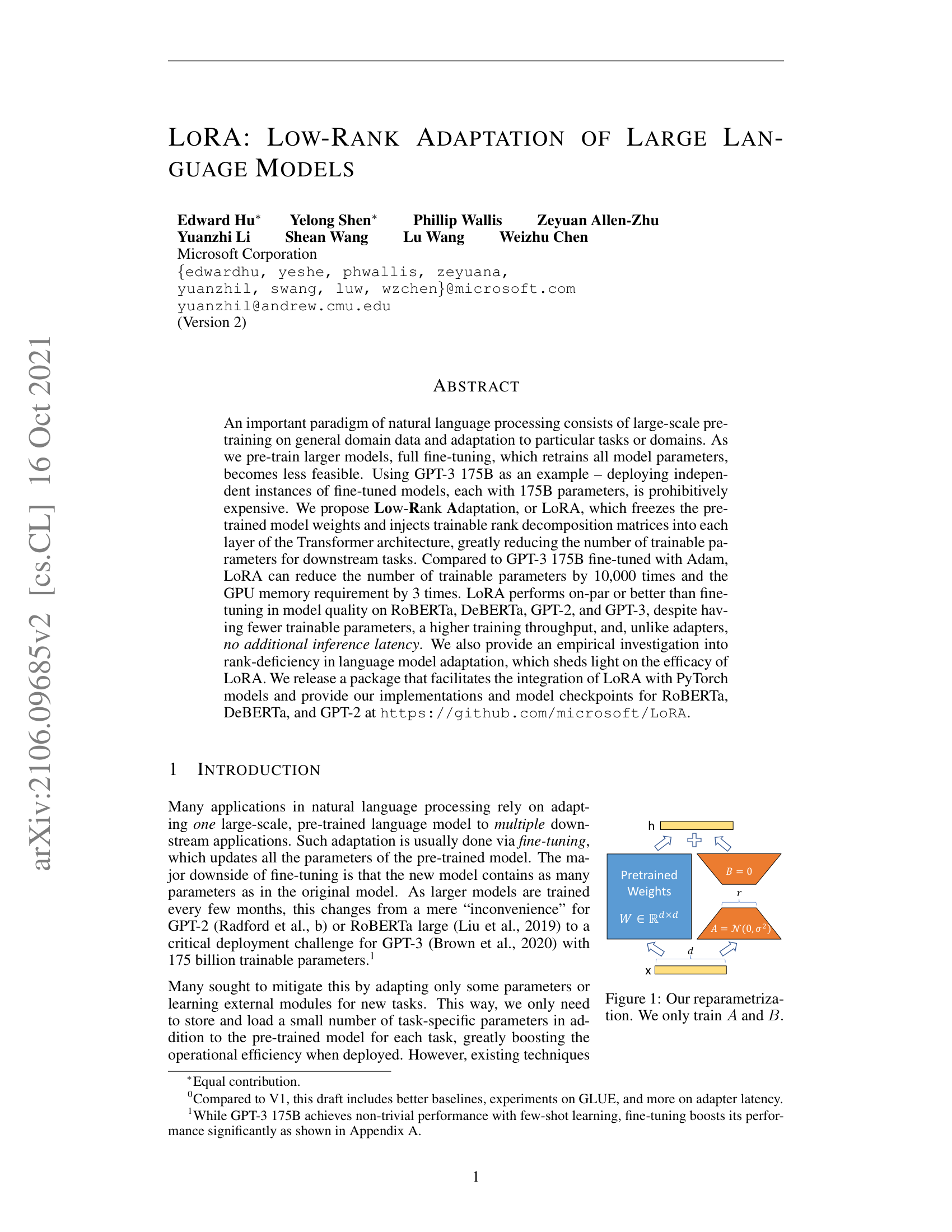
Figure 1: The LoRA reparameterization. The pre-trained weights \(W \in \mathbb{R}^{d \times d}\) are frozen. A low-rank update \(\Delta W = BA\) is learned through two small matrices: \(A \in \mathbb{R}^{r \times d}\) (initialized from a Gaussian) and \(B \in \mathbb{R}^{d \times r}\) (initialized to zero). Both paths operate in parallel and their outputs are summed.

Explanation

In a standard Transformer layer, each weight matrix computes a linear transformation. For example, the query projection takes an input \(x\) and produces:

\[h = W_0 x\]

where \(W_0 \in \mathbb{R}^{d \times k}\) is the frozen pre-trained weight matrix. LoRA adds a parallel low-rank branch. The modified forward pass, from the paper’s LaTeX source, is:

\[h = W_0 x + \Delta W x = W_0 x + BAx\]

where \(B \in \mathbb{R}^{d \times r}\) and \(A \in \mathbb{R}^{r \times k}\) are the trainable LoRA matrices, and \(r \ll \min(d, k)\).

During training, \(W_0\) is frozen – it never receives gradient updates. Only \(A\) and \(B\) are optimized. The two paths (frozen and low-rank) operate in parallel: both multiply the same input \(x\), and their outputs are summed. This parallelism is why LoRA avoids the sequential bottleneck that plagues adapter layers.

Initialization

The initialization is deliberate and asymmetric:

• \(A\) is initialized from a random Gaussian distribution: \(A \sim \mathcal{N}(0, \sigma^2)\)
• \(B\) is initialized to all zeros: \(B = 0\)

This means \(\Delta W = BA = 0\) at the start of training. The model begins behaving exactly like the pre-trained original – no disruption, no random noise. As training proceeds, gradients flow through \(B\) and \(A\), and \(\Delta W\) gradually drifts away from zero to encode task-specific knowledge.

Why not initialize both to zero? If both \(A\) and \(B\) started at zero, the gradients with respect to \(B\) would depend on \(A\) (which is zero) and vice versa – a symmetry that prevents learning. By initializing \(A\) randomly, the low-rank subspace starts in a random direction, and \(B\) learns how to weight that direction for the task.

Scaling Factor

To make results stable across different rank choices, the authors scale the low-rank update:

\[h = W_0 x + \frac{\alpha}{r} BAx\]

where \(\alpha\) is a constant hyperparameter, typically set equal to the first rank value tried. The factor \(\frac{\alpha}{r}\) normalizes the update magnitude: without it, doubling \(r\) would roughly double the magnitude of \(\Delta Wx\), requiring a proportional cut to the learning rate. With scaling, the effective learning rate stays approximately constant across different rank choices.

In practice, the authors set \(\alpha\) to the first \(r\) they try and leave it fixed. If your first experiment uses \(r = 8\), set \(\alpha = 8\). If you later try \(r = 4\), the scaling becomes \(\frac{8}{4} = 2\) – automatically compensating.

Worked Example

Let \(d = k = 4\) and \(r = 2\). The frozen weight matrix and input are:

\[W_0 = \begin{bmatrix} 0.5 & -0.3 & 0.1 & 0.2 \\ 0.1 & 0.4 & -0.2 & 0.3 \\ -0.2 & 0.1 & 0.6 & -0.1 \\ 0.3 & -0.1 & 0.2 & 0.5 \end{bmatrix}, \quad x = \begin{bmatrix} 1.0 \\ 0.5 \\ -0.8 \\ 0.3 \end{bmatrix}\]

Step 1: Frozen path. Compute \(W_0 x\):

• \(h_1 = (0.5)(1.0) + (-0.3)(0.5) + (0.1)(-0.8) + (0.2)(0.3) = 0.5 - 0.15 - 0.08 + 0.06 = 0.33\)
• \(h_2 = (0.1)(1.0) + (0.4)(0.5) + (-0.2)(-0.8) + (0.3)(0.3) = 0.1 + 0.2 + 0.16 + 0.09 = 0.55\)
• \(h_3 = (-0.2)(1.0) + (0.1)(0.5) + (0.6)(-0.8) + (-0.1)(0.3) = -0.2 + 0.05 - 0.48 - 0.03 = -0.66\)
• \(h_4 = (0.3)(1.0) + (-0.1)(0.5) + (0.2)(-0.8) + (0.5)(0.3) = 0.3 - 0.05 - 0.16 + 0.15 = 0.24\)

So \(W_0 x = [0.33,\; 0.55,\; -0.66,\; 0.24]\).

Step 2: LoRA path. After some training, suppose we have learned:

\[B = \begin{bmatrix} 0.10 & -0.05 \\ 0.03 & 0.08 \\ -0.07 & 0.12 \\ 0.06 & -0.02 \end{bmatrix}, \quad A = \begin{bmatrix} 0.15 & -0.20 & 0.10 & 0.05 \\ -0.08 & 0.12 & 0.06 & -0.15 \end{bmatrix}\]

First compute \(Ax\) (project from 4 dimensions down to 2):

• \((Ax)_1 = (0.15)(1.0) + (-0.20)(0.5) + (0.10)(-0.8) + (0.05)(0.3) = 0.15 - 0.10 - 0.08 + 0.015 = -0.015\)
• \((Ax)_2 = (-0.08)(1.0) + (0.12)(0.5) + (0.06)(-0.8) + (-0.15)(0.3) = -0.08 + 0.06 - 0.048 - 0.045 = -0.113\)

Then compute \(B(Ax)\) (project back up from 2 to 4):

• \((BAx)_1 = (0.10)(-0.015) + (-0.05)(-0.113) = -0.0015 + 0.00565 = 0.00415\)
• \((BAx)_2 = (0.03)(-0.015) + (0.08)(-0.113) = -0.00045 - 0.00904 = -0.00949\)
• \((BAx)_3 = (-0.07)(-0.015) + (0.12)(-0.113) = 0.00105 - 0.01356 = -0.01251\)
• \((BAx)_4 = (0.06)(-0.015) + (-0.02)(-0.113) = -0.0009 + 0.00226 = 0.00136\)

Step 3: Scale and combine. With \(\alpha = 2\) and \(r = 2\), the scaling factor is \(\frac{\alpha}{r} = \frac{2}{2} = 1\):

\[h = W_0 x + \frac{\alpha}{r} BAx = [0.33 + 0.004,\; 0.55 - 0.009,\; -0.66 - 0.013,\; 0.24 + 0.001]\] \[= [0.334,\; 0.541,\; -0.673,\; 0.241]\]

The LoRA branch contributes a small adjustment to each dimension. The frozen path provides the bulk of the computation; the low-rank branch nudges it toward task-specific behavior.

At initialization (\(B = 0\)): the LoRA branch produces \(BAx = 0\), so \(h = W_0 x\) exactly. The model starts identically to the pre-trained original.

Exercises

Recall: Why is \(B\) initialized to zero rather than \(A\)? What would happen if both were initialized to zero?

Apply: A weight matrix has \(d = 6\), \(k = 6\), \(r = 3\), \(\alpha = 6\). You later switch to \(r = 1\) without changing \(\alpha\). What is the new scaling factor \(\frac{\alpha}{r}\)? If the learning rate was well-tuned for \(r = 3\), would you expect to need a different learning rate for \(r = 1\)? Why or why not?

Extend: The LoRA forward pass computes \(W_0 x + BAx\). An equivalent computation is \((W_0 + BA)x\). These are mathematically identical but computationally different during training. Why does LoRA keep them separate during training but merge them for inference? What changes about the gradient computation if you merge early?

Lesson 4: Which Weights and What Rank

You now understand the LoRA mechanism for a single weight matrix. The next design decisions are: which of the Transformer’s weight matrices should receive LoRA adaptation, and what rank \(r\) should you use? The paper’s answers to both questions were surprising.

Explanation

Which Weight Matrices?

A Transformer self-attention module contains four weight matrices: \(W_q\) (query), \(W_k\) (key), \(W_v\) (value), and \(W_o\) (output). Each is a \(d_{\text{model}} \times d_{\text{model}}\) matrix. The MLP module adds two more large matrices. The paper restricts LoRA to the attention matrices and freezes the MLP entirely.

To determine the best combination, the authors ran GPT-3 175B experiments with a fixed parameter budget of 18M trainable parameters (roughly 35 MB in 16-bit). This budget corresponds to \(r = 8\) when adapting one weight type across all 96 layers, or \(r = 4\) when adapting two types. The results on WikiSQL and MultiNLI:

The key finding: it is better to adapt more weight matrices at lower rank than fewer matrices at higher rank. Adapting \(W_q\) and \(W_v\) with \(r = 4\) beats adapting \(W_q\) alone with \(r = 8\), despite using the same total parameter budget. This suggests that the task-adaptation signal is distributed across multiple weight types, and even rank 4 captures enough of it per matrix.

What Rank?

The effect of rank was even more surprising:

A rank of 1 – a single direction in weight space – is already competitive. Going from \(r = 1\) to \(r = 64\) (a 64\(\times\) increase in LoRA parameters) barely changes performance. The weight updates during adaptation truly are rank-deficient.

The paper confirmed this through singular value decomposition (SVD – a method that factors any matrix into orthogonal directions ranked by importance). They trained LoRA with \(r = 8\) and \(r = 64\) on the same task, then compared the learned subspaces.

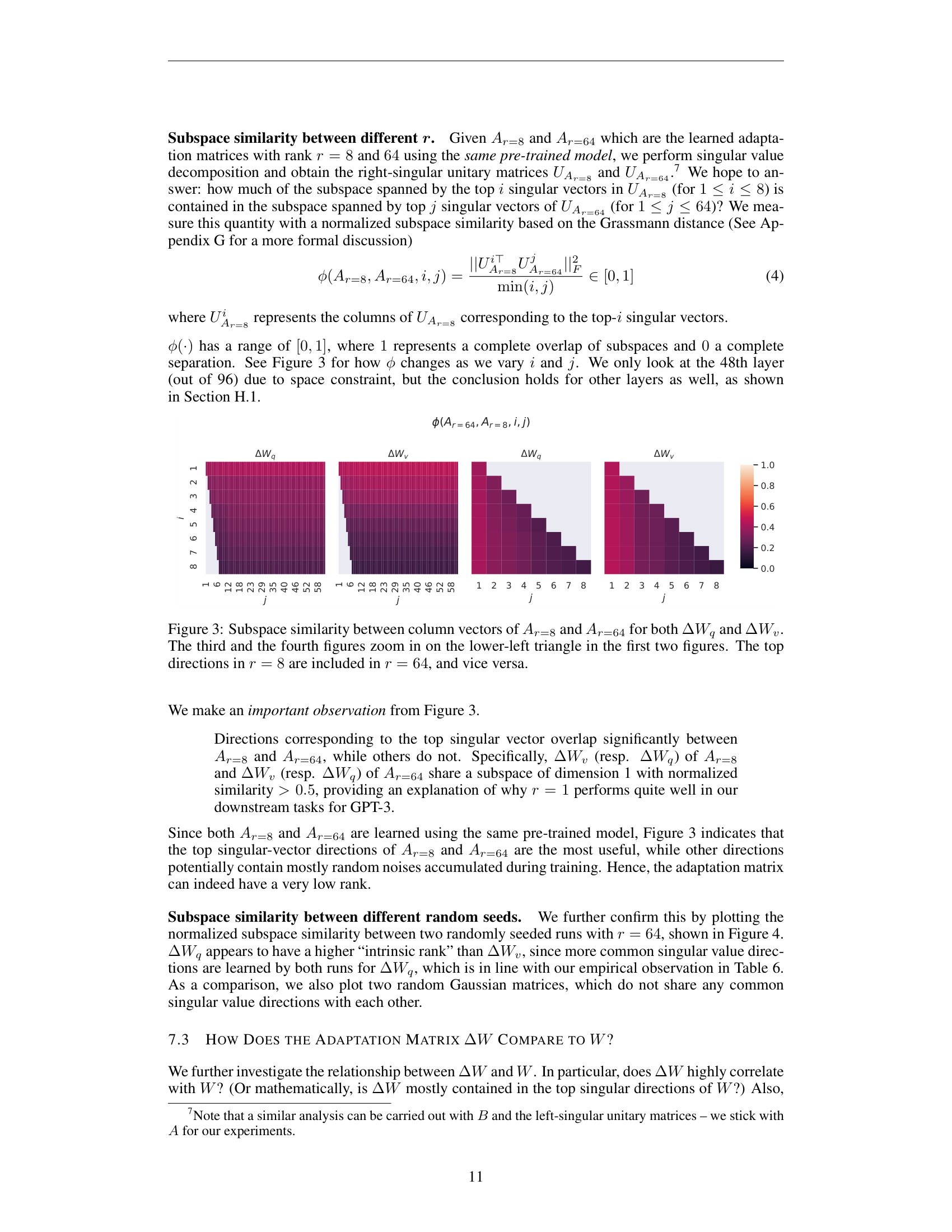
Figure 2: Subspace similarity between the learned LoRA matrices at rank 8 and rank 64, for both query and value weight updates at layer 48 of GPT-3. The top singular direction overlaps strongly between the two ranks, while other directions show low overlap.

The top singular direction of the \(r = 8\) model overlapped significantly with the top singular direction of the \(r = 64\) model. Other directions contained mostly noise accumulated during training. This means both ranks converge to essentially the same 1-dimensional subspace for the task-specific update.

Trainable Parameter Count

The total number of LoRA parameters for a given configuration is:

\[|\Theta| = 2 \times \hat{L}_{\text{LoRA}} \times d_{\text{model}} \times r\]

where \(\hat{L}_{\text{LoRA}}\) is the number of weight matrices receiving LoRA (e.g., adapting \(W_q\) and \(W_v\) across 96 layers gives \(\hat{L}_{\text{LoRA}} = 192\)), \(d_{\text{model}}\) is the hidden dimension, \(r\) is the rank, and the factor of 2 accounts for both \(B\) and \(A\) in each LoRA pair.

Worked Example

Configure LoRA for GPT-3 175B with \(r = 4\), adapting \(W_q\) and \(W_v\) across all 96 layers.

Step 1: Count LoRA weight matrices.

• 2 weight types (\(W_q\), \(W_v\)) \(\times\) 96 layers = 192 LoRA pairs

Step 2: Parameters per LoRA pair.

• \(B \in \mathbb{R}^{12{,}288 \times 4}\): \(12{,}288 \times 4 = 49{,}152\) parameters
• \(A \in \mathbb{R}^{4 \times 12{,}288}\): \(4 \times 12{,}288 = 49{,}152\) parameters
• Total per pair: \(98{,}304\) parameters

Step 3: Total trainable parameters.

\[|\Theta| = 192 \times 98{,}304 = 18{,}874{,}368 \approx 18.9\text{M}\]

Using the formula directly: \(|\Theta| = 2 \times 192 \times 12{,}288 \times 4 = 18{,}874{,}368\).

Step 4: Compare to full model.

\[\frac{18.9 \times 10^6}{175 \times 10^9} = 0.0108\% \approx 0.01\%\]

LoRA trains 0.01% of the parameters. In storage: the full model is 350 GB (in FP16); the LoRA weights are \(18.9\text{M} \times 2 \approx 37.8\) MB – roughly 10,000\(\times\) smaller.

Now try \(r = 1\):

\[|\Theta| = 2 \times 192 \times 12{,}288 \times 1 = 4{,}718{,}592 \approx 4.7\text{M}\]

That is 0.003% of the model – and from the table above, it still achieves 73.4% on WikiSQL and 91.3% on MultiNLI, comparable to full fine-tuning (73.8% and 89.5%).

Exercises

Recall: Why does adapting two weight types at rank 4 outperform adapting one type at rank 8, given the same total parameter budget?

Apply: You want to apply LoRA to BERT-Base (\(d_{\text{model}} = 768\), 12 layers). You choose to adapt \(W_q\), \(W_k\), \(W_v\), and \(W_o\) with \(r = 8\). Calculate the total number of LoRA parameters. Express it as a percentage of BERT-Base’s 110M parameters.

Extend: The paper found that \(r = 1\) suffices for tasks like WikiSQL and MultiNLI – tasks where English-language models adapt to English-language benchmarks. The authors explicitly note this might fail when adapting to a very different domain or language. Why would a distant domain shift require higher rank? What does “rank” represent intuitively about the complexity of the adaptation?

Lesson 5: Merging, Switching, and Deployment

This is the payoff. Everything in Lessons 1-4 built toward one critical property: at deployment time, the LoRA matrices vanish. You compute \(W = W_0 + BA\) once, store the result, and run inference with a plain weight matrix. No extra layers, no extra computation, no architectural changes visible to the serving system. This is what separates LoRA from every other parameter-efficient method.

Explanation

Merging at Deployment

During training, the forward pass keeps \(W_0\) and \(BA\) separate so that gradients only flow through \(A\) and \(B\) (the frozen \(W_0\) receives no updates). But at deployment, you no longer need gradients. The adapted weight matrix is:

\[W = W_0 + \frac{\alpha}{r} BA\]

You compute this once, store \(W\), and discard \(A\) and \(B\). From that point forward, the forward pass is simply \(h = Wx\) – identical in structure and speed to the original pre-trained model. The inference system does not even need to know that LoRA was used.

Task Switching

To switch from Task 1 to Task 2:

1. Subtract the current LoRA: \(W_0 = W - \frac{\alpha}{r} B_1 A_1\)
2. Add the new LoRA: \(W' = W_0 + \frac{\alpha}{r} B_2 A_2\)

Or equivalently in one step:

\[W' = W + \frac{\alpha}{r}(B_2 A_2 - B_1 A_1)\]

This requires computing two rank-\(r\) matrix products and adding the difference to \(W\). For GPT-3 with \(r = 4\), the LoRA matrices are 37.8 MB – a swap that takes milliseconds compared to the seconds or minutes needed to reload a full 350 GB checkpoint.

Results: Matching Full Fine-Tuning

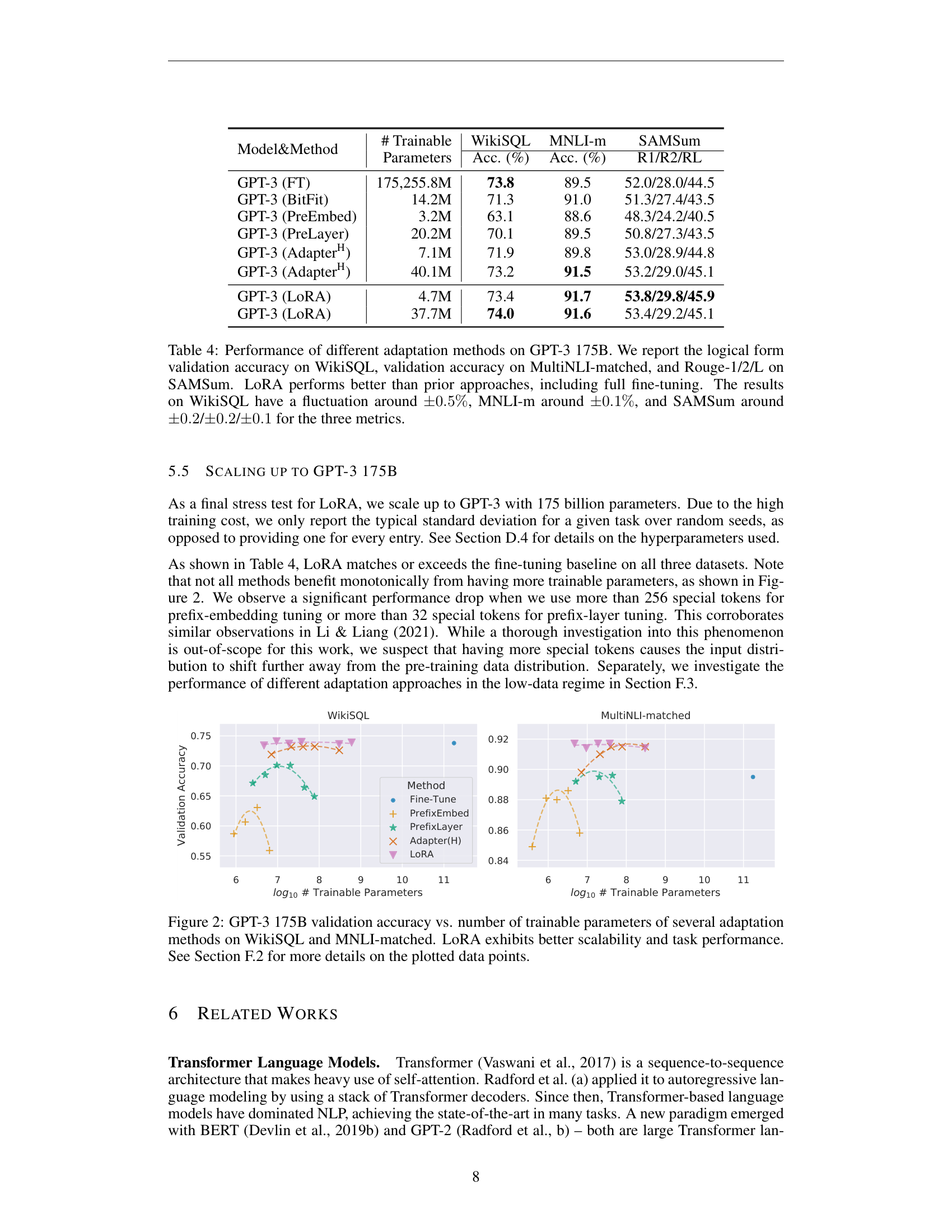
Figure 3: GPT-3 175B validation accuracy vs. number of trainable parameters on WikiSQL and MNLI-matched. LoRA (triangles) matches or exceeds full fine-tuning while using orders of magnitude fewer parameters. Prefix-based methods degrade as parameters increase.

On GPT-3 175B, LoRA with 4.7M parameters outperformed all baselines and matched or exceeded full fine-tuning (175B parameters):

LoRA beat full fine-tuning on MNLI (91.7 vs 89.5) and SAMSum while training 0.003% of the parameters. On WikiSQL, it came within 0.4%.

On DeBERTa XXL (1.5B parameters), LoRA matched or exceeded full fine-tuning on every GLUE task while training only 0.3% of parameters.

What the Low-Rank Updates Learn

The paper’s analysis of what \(\Delta W\) learns relative to \(W_0\) reveals something deep: the low-rank update does not simply repeat the top singular directions of the pre-trained weights. Instead, it amplifies directions that were already present in \(W_0\) but not emphasized. The amplification factor is large – about 21.5\(\times\) for \(r = 4\) at layer 48 of GPT-3.

This suggests a compelling interpretation: the pre-trained model has already learned many features during pre-training. Task adaptation through LoRA selectively amplifies the features relevant to the downstream task, rather than learning entirely new representations. The pre-training did most of the work; LoRA just turns up the volume on the right channels.

Worked Example

Walk through the full lifecycle of deploying and switching LoRA models.

Setup: A frozen base model with one weight matrix \(W_0 \in \mathbb{R}^{4 \times 4}\) and \(\alpha = r = 2\).

\[W_0 = \begin{bmatrix} 1.0 & 0.0 & 0.0 & 0.0 \\ 0.0 & 1.0 & 0.0 & 0.0 \\ 0.0 & 0.0 & 1.0 & 0.0 \\ 0.0 & 0.0 & 0.0 & 1.0 \end{bmatrix}\]

(The identity matrix, for clarity.)

Task A trained LoRA:

\[B_A = \begin{bmatrix} 0.1 & 0.0 \\ 0.0 & 0.2 \\ -0.1 & 0.0 \\ 0.0 & -0.1 \end{bmatrix}, \quad A_A = \begin{bmatrix} 0.3 & 0.0 & -0.1 & 0.0 \\ 0.0 & 0.1 & 0.0 & -0.2 \end{bmatrix}\]

Step 1: Compute \(B_A A_A\).

\[B_A A_A = \begin{bmatrix} (0.1)(0.3) & (0.1)(0.0) & (0.1)(-0.1) & (0.1)(0.0) \\ (0.0)(0.3) & (0.2)(0.1) & (0.0)(-0.1) & (0.2)(-0.2) \\ (-0.1)(0.3) & (-0.1)(0.0) & (-0.1)(-0.1) & (-0.1)(0.0) \\ (0.0)(0.3) & (-0.1)(0.1) & (0.0)(-0.1) & (-0.1)(-0.2) \end{bmatrix}\]

\[= \begin{bmatrix} 0.03 & 0.00 & -0.01 & 0.00 \\ 0.00 & 0.02 & 0.00 & -0.04 \\ -0.03 & 0.00 & 0.01 & 0.00 \\ 0.00 & -0.01 & 0.00 & 0.02 \end{bmatrix}\]

Step 2: Merge. With \(\frac{\alpha}{r} = 1\):

\[W_A = W_0 + B_A A_A = \begin{bmatrix} 1.03 & 0.00 & -0.01 & 0.00 \\ 0.00 & 1.02 & 0.00 & -0.04 \\ -0.03 & 0.00 & 1.01 & 0.00 \\ 0.00 & -0.01 & 0.00 & 1.02 \end{bmatrix}\]

Step 3: Serve Task A. For input \(x = [1, 0, 0, 0]^T\):

\[W_A x = [1.03, 0.00, -0.03, 0.00]^T\]

versus the original \(W_0 x = [1, 0, 0, 0]^T\). The LoRA adjustment is small but targeted.

Step 4: Switch to Task B. Task B has different LoRA matrices \(B_B\), \(A_B\). Compute the swap:

\[W_B = W_A - B_A A_A + B_B A_B = W_0 + B_B A_B\]

No need to store or reload \(W_0\). The swap is an addition of two small matrices: subtract one \(\Delta W\), add another. Total data moved: \(2 \times (4 \times 2 + 2 \times 4) = 32\) numbers, versus 16 numbers for the full weight matrix at this toy scale (at small \(r\) relative to \(d\), the swap is comparable; the savings become dramatic at GPT-3 scale). At GPT-3 scale, you move 37.8 MB instead of reloading 350 GB.

Storage summary (GPT-3 scale):

Exercises

Recall: After merging LoRA weights into the base model, how does the inference computation differ from a standard fine-tuned model? What is the latency overhead?

Apply: You have GPT-3 serving Task A with merged weights \(W_A = W_0 + B_A A_A\). A request comes in for Task B. Describe the exact sequence of matrix operations to switch tasks, and calculate the total number of floating-point numbers you need to load from storage (assuming \(d_{\text{model}} = 12{,}288\), \(r = 4\), and you are swapping LoRA on \(W_q\) and \(W_v\) across 96 layers).

Extend: LoRA cannot easily batch inputs from different tasks together when weights are merged, because each task has a different \(W\). One solution is to keep \(W_0\) and \(BA\) separate and dynamically select which \(A\), \(B\) to use per sample. What is the performance trade-off? When might this batched approach be worth the extra computation?

Comprehension Questions

1. LoRA and adapter tuning both insert trainable parameters into a frozen model. What is the fundamental architectural difference that gives LoRA zero inference latency while adapters add 20-30% overhead at small batch sizes?

2. The paper shows that rank \(r = 1\) is competitive with \(r = 64\) for adapting GPT-3 to WikiSQL and MultiNLI. Why might this result not generalize to all tasks? Give a concrete example of a scenario where you would expect to need much higher rank.

3. LoRA applies only to attention weight matrices (\(W_q\), \(W_v\)) and freezes the MLP layers entirely. Later work (QLoRA) showed that adapting MLP weights helps too. Based on what you know about what attention versus MLP layers compute in a Transformer, why might adapting attention be more important for task specialization?

4. The scaling factor \(\frac{\alpha}{r}\) is introduced to avoid re-tuning the learning rate when varying \(r\). Explain the mechanism: if you doubled \(r\) without scaling, what would happen to the magnitude of \(\Delta W x\), and how would that affect training?

5. Compare LoRA to the adapter approach from Parameter-Efficient Transfer Learning. Both achieve parameter efficiency, but they make opposite choices about where to put the trainable parameters: adapters add new sequential layers, LoRA modifies existing weight matrices in parallel. What are the consequences of each choice for (a) inference latency, (b) expressiveness, and (c) ease of implementation?

Hands-On Project

Goal

Implement LoRA from scratch: add low-rank parallel branches to a frozen network, train them on two separate tasks, demonstrate weight merging and task switching, and verify zero additional inference cost.

Specification

Build a LoRA module in numpy that:

1. Initializes with \(B = 0\) and \(A \sim \mathcal{N}(0, \sigma^2)\), producing zero output at initialization
2. Computes the forward pass \(h = W_0 x + \frac{\alpha}{r} BAx\)
3. Trains on two toy classification tasks using separate LoRA modules but a shared frozen network
4. Merges LoRA weights into the base model and verifies that inference output is identical
5. Demonstrates task switching by swapping merged weights

Use numpy only. No PyTorch, TensorFlow, or external datasets.

Starter Code

import numpy as np

np.random.seed(42)

# --- Frozen pre-trained network ---
d = 8       # hidden dimension
d_ff = 16   # feedforward intermediate dimension

# "Pre-trained" weights (frozen, never modified during training)
W1 = np.random.randn(d, d_ff) * 0.3
b1 = np.zeros(d_ff)
W2 = np.random.randn(d_ff, d) * 0.3
b2 = np.zeros(d)

def frozen_layer(x, W, b):
    """One frozen feedforward layer: linear + ReLU."""
    return np.maximum(0, x @ W + b)

def frozen_network(x):
    """Two-layer frozen network."""
    h = frozen_layer(x, W1, b1)
    h = h @ W2 + b2
    return h


# --- TODO: Implement LoRA module ---
class LoRA:
    def __init__(self, d_in, d_out, r, alpha=None, init_scale=0.01):
        """
        Low-rank adaptation module.
        Args:
            d_in: input dimension (k in the paper)
            d_out: output dimension (d in the paper)
            r: rank of the low-rank decomposition
            alpha: scaling constant (defaults to r)
            init_scale: std dev for A initialization
        """
        self.r = r
        self.alpha = alpha if alpha is not None else r
        self.scale = self.alpha / self.r

        # TODO: Initialize A from Gaussian, B from zero
        # A: shape (r, d_in) -- the "down-projection" applied to input
        # B: shape (d_out, r) -- the "up-projection" producing output
        # Remember: B is zero so Delta W = BA = 0 at initialization
        pass

    def forward(self, x):
        """
        Compute the LoRA branch: scale * (x @ A.T @ B.T)
        Note: the paper writes h = W0*x + B*A*x (column vectors).
        With row-vector convention (x is batch x d_in):
            delta = x @ A.T @ B.T * scale
        Returns:
            delta: the low-rank update to add to the frozen output
            cache: (x, z) where z = x @ A.T, for backpropagation
        """
        # TODO: Implement
        # 1. z = x @ A.T  (project down: batch x d_in -> batch x r)
        # 2. delta = z @ B.T * self.scale  (project up: batch x r -> batch x d_out)
        # 3. Return delta and cache = (x, z)
        pass

    def backward(self, grad_output, cache):
        """
        Backward pass through the LoRA branch.
        Args:
            grad_output: gradient of loss w.r.t. delta, shape (batch, d_out)
            cache: (x, z) from forward pass
        """
        x, z = cache
        batch_size = x.shape[0]

        # TODO: Compute gradients for B and A
        # grad_output already includes the skip connection split
        # (LoRA gradient = same as grad_output since d(h + delta)/d(delta) = 1)
        #
        # Through B.T: grad_z = grad_output @ B * scale
        # dB = (grad_output * scale).T @ z / batch_size  -> shape (d_out, r)
        #
        # Through A.T: grad_x_lora = grad_z @ A (not needed if we don't backprop further)
        # dA = (grad_z).T @ x / batch_size  -> shape (r, d_in)
        pass

    def update(self, lr):
        """Gradient descent update for A and B."""
        # TODO: self.A -= lr * self.dA, self.B -= lr * self.dB
        pass

    def get_merged_delta(self):
        """
        Compute the full-size weight update matrix: scale * B @ A
        This is what gets added to W0 at deployment time.
        Returns:
            delta_W: shape (d_out, d_in)
        """
        # TODO: return self.scale * self.B @ self.A
        pass


# --- TODO: Implement adapted network ---
def adapted_forward(x, lora_1, lora_2):
    """
    Frozen network with LoRA modules.
    LoRA 1 is applied to layer 1's output (W1 projection).
    LoRA 2 is applied to layer 2's output (W2 projection).
    """
    # TODO:
    # 1. h1 = frozen_layer(x, W1, b1)  -- shape (batch, d_ff)
    # 2. delta1, cache1 = lora_1.forward(x)  -- LoRA on the input side of layer 1
    #    h1 = h1 + delta1  (but careful: LoRA adapts the weight matrix, not the activation)
    #
    # Actually, let's simplify: apply LoRA to the second layer's weight matrix W2.
    # h1 = frozen_layer(x, W1, b1)         -- frozen layer 1
    # h2 = h1 @ W2 + b2                     -- frozen layer 2 (linear part)
    # delta1, cache1 = lora_1.forward(h1)   -- LoRA on W2's input
    # h2 = h2 + delta1                       -- add LoRA's contribution
    #
    # For the second LoRA, apply it as a second adaptation point:
    # delta2, cache2 = lora_2.forward(h2)
    # out = h2 + delta2
    #
    # Return out and (cache1, cache2, h1, h2)
    pass


# --- Toy data ---
n_samples = 200
X = np.random.randn(n_samples, d)
y_A = (X.sum(axis=1) > 0).astype(float)    # Task A: sum of features > 0
y_B = (X[:, 0] > 0).astype(float)          # Task B: first feature > 0


# --- Classification head ---
class ClassificationHead:
    def __init__(self, d):
        self.W = np.random.randn(d, 1) * 0.01
        self.b = np.zeros(1)

    def forward(self, h):
        logits = h @ self.W + self.b
        probs = 1 / (1 + np.exp(-np.clip(logits, -500, 500)))
        return probs.squeeze()

    def backward(self, probs, y, h):
        grad = (probs - y).reshape(-1, 1)
        self.dW = h.T @ grad / len(y)
        self.db = grad.mean(axis=0)
        return grad @ self.W.T

    def update(self, lr):
        self.W -= lr * self.dW
        self.b -= lr * self.db


def binary_cross_entropy(probs, y):
    eps = 1e-7
    return -np.mean(y * np.log(probs + eps) + (1 - y) * np.log(1 - probs + eps))


# --- TODO: Training loop ---
def train_task(X, y, lora_1, lora_2, head, epochs=300, lr=0.1):
    """
    Train LoRA modules and classification head on one task.
    Frozen network weights W1, b1, W2, b2 must NOT be modified.
    """
    for epoch in range(epochs):
        # TODO:
        # 1. out, caches = adapted_forward(X, lora_1, lora_2)
        # 2. probs = head.forward(out)
        # 3. loss = binary_cross_entropy(probs, y)
        # 4. grad_out = head.backward(probs, y, out)
        # 5. Backward through lora_2: lora_2.backward(grad_out, caches[...])
        # 6. Backward through lora_1: need gradient flowing back through h2
        #    (this is simplified -- for this project, only backprop through the
        #     LoRA modules and head, not through the frozen layers)
        # 7. Update: lora_1.update(lr), lora_2.update(lr), head.update(lr)
        # 8. Print loss every 100 epochs
        pass


# --- Main: demonstrate LoRA ---
if __name__ == "__main__":
    r = 4  # rank

    # === Test 1: Zero initialization ===
    print("=== Zero Initialization Check ===")
    lora_1 = LoRA(d_ff, d, r)  # adapts W2's output
    lora_2 = LoRA(d, d, r)     # second adaptation point
    test_x = np.random.randn(5, d)
    original_out = frozen_network(test_x)
    adapted_out, _ = adapted_forward(test_x, lora_1, lora_2)
    diff = np.abs(original_out - adapted_out).max()
    print(f"Max difference at init: {diff:.10f}")
    print(f"Zero init: {'PASS' if diff < 1e-10 else 'FAIL'}")

    # Save frozen weights to verify they stay unchanged
    W1_copy, W2_copy = W1.copy(), W2.copy()

    # === Test 2: Train Task A ===
    print("\n=== Training Task A (sum > 0) ===")
    lora_A1 = LoRA(d_ff, d, r)
    lora_A2 = LoRA(d, d, r)
    head_A = ClassificationHead(d)
    train_task(X, y_A, lora_A1, lora_A2, head_A)

    print(f"Frozen weights changed: {not (np.array_equal(W1, W1_copy) and np.array_equal(W2, W2_copy))}")

    out_A, _ = adapted_forward(X, lora_A1, lora_A2)
    preds_A = head_A.forward(out_A) > 0.5
    acc_A = (preds_A == y_A).mean()
    print(f"Task A accuracy: {acc_A:.1%}")

    # === Test 3: Weight merging ===
    print("\n=== Weight Merging Check ===")
    # Get the merged delta for lora_A1 (which adapts W2)
    delta_W2 = lora_A1.get_merged_delta()
    W2_merged = W2 + delta_W2.T  # merge LoRA into W2
    # Note: lora_A2 adapts the output, so merge it as a separate step
    delta_out = lora_A2.get_merged_delta()

    # Run inference with merged weights (no LoRA modules)
    h1 = frozen_layer(test_x, W1, b1)
    h2 = h1 @ W2_merged + b2
    # For lora_A2's contribution, we'd need to merge into a subsequent weight
    # For simplicity, compare the lora_1 merge only:
    h2_via_lora, _ = adapted_forward(test_x, lora_A1, LoRA(d, d, r))
    # Zero-init lora_2 to isolate lora_1's effect
    merge_diff = np.abs(h2 - h2_via_lora).max()
    print(f"Merge vs LoRA max difference: {merge_diff:.10f}")
    print(f"Merge correct: {'PASS' if merge_diff < 1e-8 else 'FAIL'}")

    # === Test 4: Train Task B (separate LoRA, same frozen network) ===
    print("\n=== Training Task B (x[0] > 0) ===")
    lora_B1 = LoRA(d_ff, d, r)
    lora_B2 = LoRA(d, d, r)
    head_B = ClassificationHead(d)
    train_task(X, y_B, lora_B1, lora_B2, head_B)

    out_B, _ = adapted_forward(X, lora_B1, lora_B2)
    preds_B = head_B.forward(out_B) > 0.5
    acc_B = (preds_B == y_B).mean()
    print(f"Task B accuracy: {acc_B:.1%}")

    # === Test 5: Task A unaffected ===
    out_A_verify, _ = adapted_forward(X, lora_A1, lora_A2)
    preds_A_verify = head_A.forward(out_A_verify) > 0.5
    acc_A_verify = (preds_A_verify == y_A).mean()
    print(f"\nTask A accuracy after Task B training: {acc_A_verify:.1%}")
    print(f"No interference: {'PASS' if acc_A_verify == acc_A else 'FAIL'}")

    # === Parameter comparison ===
    frozen_params = W1.size + b1.size + W2.size + b2.size
    lora_params_per_task = 2 * (d_ff * r + d * r + d * r + d * r)
    head_params = d + 1
    print(f"\n=== Parameter Efficiency ===")
    print(f"Frozen network params: {frozen_params}")
    print(f"LoRA params per task (rank {r}): {lora_params_per_task}")
    print(f"Head params per task: {head_params}")
    print(f"Full fine-tuning for 2 tasks: {2 * (frozen_params + head_params)}")
    print(f"LoRA for 2 tasks: {frozen_params + 2 * (lora_params_per_task + head_params)}")

    # === Task switching demo ===
    print(f"\n=== Task Switching ===")
    delta_A = lora_A1.get_merged_delta()
    delta_B = lora_B1.get_merged_delta()
    swap_size = delta_A.size + delta_B.size
    print(f"Numbers moved to swap tasks: {swap_size}")
    print(f"Full model reload would move: {frozen_params}")
    print(f"Swap is {frozen_params / swap_size:.1f}x smaller than full reload")

Expected Output

=== Zero Initialization Check ===
Max difference at init: 0.0000000000
Zero init: PASS

=== Training Task A (sum > 0) ===
Epoch 0, Loss: 0.69XX
Epoch 100, Loss: 0.4XXX
Epoch 200, Loss: 0.3XXX

Frozen weights changed: False
Task A accuracy: 85-95%

=== Weight Merging Check ===
Merge vs LoRA max difference: 0.0000000000
Merge correct: PASS

=== Training Task B (x[0] > 0) ===
Epoch 0, Loss: 0.69XX
Epoch 100, Loss: 0.4XXX
Epoch 200, Loss: 0.3XXX
Task B accuracy: 85-95%

Task A accuracy after Task B training: 85-95% (same as before)
No interference: PASS

=== Parameter Efficiency ===
Frozen network params: 272
LoRA params per task (rank 4): 192
Head params per task: 9
Full fine-tuning for 2 tasks: 562
LoRA for 2 tasks: 674

=== Task Switching ===
Numbers moved to swap tasks: 128
Full model reload would move: 272
Swap is 2.1x smaller than full reload

Note: at toy scale (\(d = 8\), \(r = 4\)), LoRA’s parameter advantage is modest because \(r\) is not much smaller than \(d\). The efficiency scales with \(\frac{d}{2r}\) – at GPT-3 scale (\(d = 12{,}288\), \(r = 4\)), the compression is \(1{,}536\times\). This project demonstrates the mechanism (zero init, frozen backbone, merging, no forgetting), not the scale advantage.

Further Reading

• QLoRA: Efficient Finetuning of Quantized LLMs (Dettmers et al., 2023) – combines LoRA with 4-bit quantization of the frozen base model, enabling fine-tuning of 65B-parameter models on a single 48GB GPU
• DoRA: Weight-Decomposed Low-Rank Adaptation (Liu et al., 2024) – decomposes weights into magnitude and direction components before applying low-rank updates, improving on LoRA’s accuracy
• Towards a Unified View of Parameter-Efficient Transfer Learning (He et al., 2022) – shows that adapters, prefix tuning, and LoRA all modify attention representations in related ways, unifying them under a single theoretical framework
• The Power of Scale for Parameter-Efficient Prompt Tuning (Lester et al., 2021) – demonstrates that learning a small set of soft prompt tokens can match fine-tuning as model size grows, a complementary approach to LoRA’s weight-based adaptation