Lost in the Middle: How Language Models Use Long Contexts – Course

Learning Objectives

By the end of this course, you will be able to:

1. Explain how context windows work in Transformer-based language models and why position within the window matters
2. Design controlled experiments that isolate a model’s sensitivity to the position of relevant information
3. Interpret the U-shaped performance curve and define primacy bias and recency bias in the context of language models
4. Compare how decoder-only and encoder-decoder architectures handle positional information and explain why bidirectional attention helps
5. Evaluate the trade-off between retrieval recall and reader accuracy in retrieval-augmented generation (RAG) systems
6. Apply the paper’s findings to design better context layouts for production RAG pipelines

Prerequisites

• Transformer architecture – how self-attention lets every token attend to other tokens, the difference between encoder (bidirectional) and decoder (causal/left-to-right) attention masks. Covered in the Transformers course (see Attention Is All You Need).
• Autoregressive language models – how decoder-only models generate text one token at a time, each conditioned on all previous tokens. Covered in the GPT course (see Improving Language Understanding by Generative Pre-Training).
• Retrieval-augmented generation (RAG) – the pattern of retrieving documents from a corpus and injecting them into a language model’s prompt to answer questions. Covered in the RAG course (see Retrieval-Augmented Generation).
• Basic probability – accuracy, recall, conditional probability, indicator functions.

Lesson 1: Context Windows – What the Model Sees

Every language model has a limit on how much text it can process at once. That limit determines what the model can “see” when you ask it a question. Before you can understand how models use their input, you need to understand what their input looks like.

Explanation

Think of a model’s context window as a desk. The desk has a fixed width, and you can spread documents across it. A small desk fits three pages; a large desk fits fifty. In both cases, the model reads everything on the desk before generating an answer. But here is the question this paper asks: does the model read every page on the desk with equal care, or does it skim some and study others?

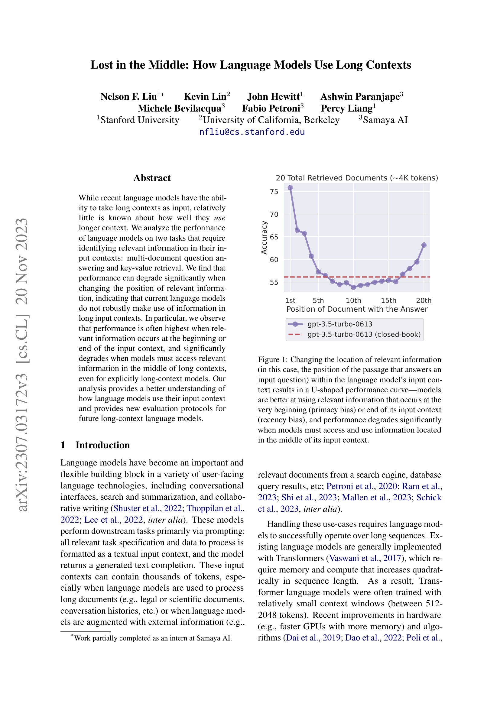
Figure 1: The paper’s central finding. Accuracy is highest when the relevant document is at the beginning or end of the input, and drops sharply in the middle – forming a U-shaped curve across all tested models.

A context window is the maximum number of tokens (roughly, word fragments) a model can accept as input. In mid-2023, context window sizes varied widely:

Transformer models process input through self-attention (see Attention Is All You Need). In a decoder-only model like GPT, each token can only attend to tokens that came before it – this is called causal or left-to-right attention. Token 500 can look back at tokens 1 through 499, but not forward to token 501. In an encoder-decoder model like T5, the encoder is bidirectional: every token attends to every other token simultaneously.

This asymmetry matters for how information at different positions gets processed. In a decoder-only model, a question placed at the end of the context can attend to all preceding documents. But those documents, processed earlier, never “see” the question – they are contextualized without knowing what the model will be asked. An encoder-decoder model does not have this limitation: every document token can attend to the question token, regardless of position.

Positional encoding tells the model where each token sits in the sequence. Different models use different schemes – absolute learned embeddings, ALiBi (Attention with Linear Biases), rotary positional embeddings (which encode position by rotating the query and key vectors by an angle proportional to their position) – but they all serve the same purpose: allowing the model to distinguish “token at position 5” from “token at position 5,000.” The paper does not study which positional encoding works best, but the choice of encoding affects how well models generalize to positions they rarely encountered during training.

Worked Example

Suppose you are building a question-answering system. Your model has a 4,096-token context window, and you retrieve 20 Wikipedia passages of approximately 100 tokens each. Let’s compute the input layout:

System instruction:       ~50 tokens
20 documents x 100 tokens: ~2,000 tokens
Document formatting:       ~200 tokens  (titles, "[Document 1]:" markers, etc.)
Question:                  ~20 tokens
Total:                     ~2,270 tokens

This fits within the 4K window. Now, the document that actually answers the question could be placed at any of the 20 positions. If it is Document 1, it sits near the start of the context (around token 50). If it is Document 10, it sits in the middle (around token 1,100). If it is Document 20, it sits near the end (around token 2,050), just before the question.

In a decoder-only model, when the model processes Document 1, it has not yet seen the question (which appears at the end). When it processes Document 20, the question is still ahead of it. Only after all documents are processed and the question appears do the attention layers get to “look back” at the documents when generating the answer.

Exercises

Recall: What is the difference between a decoder-only model’s attention and an encoder-decoder model’s encoder attention? Which one allows every token to attend to every other token?

Apply: A model has a context window of 8,192 tokens. You need to include a system prompt (80 tokens), a question (30 tokens), and retrieved documents. Each document is approximately 120 tokens, with 15 tokens of formatting overhead per document. How many documents can you fit? Show your calculation.

Extend: Two models have the same 16K context window, but one was trained on sequences of 2K tokens and then adapted to 16K, while the other was trained on 16K sequences from the start. Both technically accept 16K tokens. Would you expect them to handle information at position 15,000 equally well? Why or why not?

Lesson 2: The Serial-Position Effect – A Clue from Human Memory

Before diving into the experimental results, it helps to know that the pattern the paper discovers has a well-studied parallel in psychology. Humans have a remarkably predictable blind spot when recalling items from a list – and language models turn out to share it.

Explanation

In the 1960s, psychologist Bennet Murdock ran a simple experiment. He read lists of words aloud to participants, then asked them to recall as many words as possible. The result was strikingly consistent: people remembered the first few words well (the primacy effect), remembered the last few words well (the recency effect), and performed worst on words in the middle.

Plotted on a graph with list position on the x-axis and recall probability on the y-axis, this produces a U-shaped curve. Psychologists call this the serial-position effect, first described by Hermann Ebbinghaus in 1913.

The standard explanation involves two memory systems. Items at the beginning of the list get rehearsed more (they enter long-term memory). Items at the end are still fresh in short-term (working) memory. Items in the middle get neither advantage – they were pushed out of short-term memory by subsequent items and did not get enough rehearsal to enter long-term memory.

Now consider a language model processing 20 documents. The model has no “short-term” or “long-term” memory in the human sense – it has self-attention, which can theoretically attend equally to any position. Yet the paper shows that these models exhibit the same U-shaped pattern: they perform best when critical information is at the beginning or end of the context, and worst when it is in the middle.

This is surprising precisely because it shouldn’t happen. The attention mechanism in a Transformer computes:

\[\text{Attention}(Q, K, V) = \text{softmax}\left(\frac{QK^T}{\sqrt{d_k}}\right)V\]

where:

• \(Q\) is the matrix of query vectors (one per token generating output)
• \(K\) is the matrix of key vectors (one per token being attended to)
• \(V\) is the matrix of value vectors (the content being retrieved)
• \(d_k\) is the dimension of the key vectors
• The softmax normalizes attention weights so they sum to 1

Nothing in this formula privileges any position. The dot product \(QK^T\) depends on the content of the queries and keys, not their position in the sequence (positional information is added separately through encodings). So any positional bias the model exhibits must come from how it was trained – from patterns in the training data and the interaction between learned weights and positional encodings – not from the architecture itself.

Worked Example

Imagine a simplified scenario with 5 documents and an attention mechanism. After the softmax, the model assigns these attention weights to each document when generating the answer:

The answer-containing document gets only 5% of the attention – the model barely looks at position 3. Even though Document 3 contains the information needed to answer the question, the model allocates most of its attention to the beginning (30%) and end (40%). This U-shaped distribution of attention weights produces the U-shaped accuracy curve the paper measures.

Now imagine we move the answer document to position 1:

Now the answer gets 30% of attention – six times more than when it was in the middle. The model is much more likely to extract and use the answer correctly.

Exercises

Recall: What are the two components of the serial-position effect in human memory, and what is the analogous U-shaped pattern observed in language models?

Apply: Given attention weights [0.25, 0.12, 0.08, 0.06, 0.07, 0.09, 0.13, 0.20] for 8 documents, which positions get the most attention? Compute the ratio of attention at position 1 versus position 4. If the answer document were at position 4, what fraction of attention would it receive?

Extend: The attention formula has no inherent positional preference, yet models show a strong position bias. The paper hypothesizes this comes from training data patterns (e.g., StackOverflow posts where important information appears at the beginning). What other training data patterns might contribute to primacy or recency bias? Consider what kinds of text dominate web-scale training corpora.

Lesson 3: Measuring Position Sensitivity – The Experimental Method

Knowing that a bias might exist is different from proving it does. This lesson covers how the authors designed controlled experiments that isolate the effect of information position from everything else – a method that became a standard evaluation protocol for long-context models.

Explanation

Think of this like a hearing test. An audiologist does not play a song and ask “can you hear?” Instead, they play a single tone at a precise frequency and volume, then systematically vary each parameter while holding others constant. This controlled approach lets them map out exactly where hearing is strong and where it drops off.

The paper applies the same logic to language model context usage. The authors design two tasks where they can precisely control two variables:

1. Where in the context the relevant information appears (position)
2. How long the total context is (number of documents or key-value pairs)

Everything else stays fixed: the question, the answer, the distractor documents (irrelevant documents included to pad the context), the prompt format, the decoding method (greedy decoding, where the model always picks the single most probable next token), and the evaluation metric.

Task 1: Multi-Document Question Answering. The model receives \(k\) documents and a question. Exactly one document contains the answer; the other \(k - 1\) are distractors retrieved by Contriever (a neural search engine that encodes queries and documents as vectors and ranks by similarity) that are topically relevant but do not contain the answer. The authors test \(k \in \{10, 20, 30\}\), corresponding to approximately 2K, 4K, and 6K tokens.

The key manipulation: the authors slide the answer-containing document from position 1 to position \(k\), running the full evaluation at each position. This produces one accuracy measurement per position.

Task 2: Synthetic Key-Value Retrieval. To separate information location from language understanding, the authors create a minimal retrieval task: a JSON object with \(k\) key-value pairs (all random 128-bit UUIDs – Universally Unique Identifiers, long random hexadecimal strings like 550e8400-e29b-41d4-a716-446655440000) and a query asking for the value of a specific key. No natural language comprehension is needed – the model just has to find a matching string and copy the associated value. They test \(k \in \{75, 140, 300\}\), corresponding to approximately 4K, 8K, and 16K tokens.

Accuracy metric. Both tasks use the same metric:

\[\text{Accuracy} = \frac{1}{N} \sum_{i=1}^{N} \mathbf{1}[\text{answer}_i \in \text{output}_i]\]

where:

• \(N\) is the number of evaluation examples (2,655 for QA, 500 for key-value retrieval)
• \(\text{answer}_i\) is any of the gold-standard correct answers for example \(i\)
• \(\text{output}_i\) is the model’s generated text for example \(i\)
• \(\mathbf{1}[\cdot]\) is the indicator function: returns 1 if the condition is true, 0 otherwise
• The \(\in\) check is a substring match – the correct answer must appear somewhere in the model’s output

This accuracy is then conditioned on position. The paper’s central measurement is:

\[\text{Accuracy}(p) = \frac{1}{|\{i : \text{pos}(r_i) = p\}|} \sum_{i : \text{pos}(r_i) = p} \mathbf{1}[\text{answer}_i \in \text{output}_i]\]

where:

• \(p\) is the position of the relevant document (or key-value pair) in the input, ranging from 1 to \(k\)
• \(\text{pos}(r_i)\) is the position of the relevant information in example \(i\)
• The sum counts only examples where the answer is at position \(p\)

If a model uses its context uniformly, \(\text{Accuracy}(p)\) should be roughly flat across all positions. Any variation reveals positional bias.

The authors also compare against two baselines. Closed-book: the model answers without any documents (testing parametric knowledge – facts the model absorbed during pretraining and stored in its weights – alone). Oracle: the model receives only the single document containing the answer (testing comprehension without the distraction of other documents).

Worked Example

Let’s walk through how position-conditioned accuracy is computed. Suppose we have 10 evaluation examples and 5 documents (\(k = 5\)). We run the experiment with the answer at each position (2 examples per position):

Position-conditioned accuracy:

• \(\text{Accuracy}(1) = (1 + 0) / 2 = 50\%\)
• \(\text{Accuracy}(2) = (0 + 1) / 2 = 50\%\)
• \(\text{Accuracy}(3) = (0 + 0) / 2 = 0\%\)
• \(\text{Accuracy}(4) = (1 + 1) / 2 = 100\%\)
• \(\text{Accuracy}(5) = (1 + 1) / 2 = 100\%\)

This toy example shows a recency-dominant pattern (accuracy rises toward the end). With 2,655 examples per position (the actual paper), the curves are much smoother and the U-shape is unmistakable.

Exercises

Recall: Why does the paper use two different tasks (multi-document QA and key-value retrieval)? What does the key-value task test that the QA task does not isolate?

Apply: You have 100 evaluation examples and 10 document positions. You want to compute position-conditioned accuracy with 10 examples per position. If position 5 yields correct answers on examples 41, 43, 46, and 49 (out of examples 41-50), what is \(\text{Accuracy}(5)\)? Is this better or worse than the paper’s finding for mid-positions with 20 documents?

Extend: The paper uses “substring match” as its accuracy criterion – the correct answer just needs to appear somewhere in the model’s output. What are the advantages and disadvantages of this metric compared to exact match? Can you think of a scenario where substring match would give a false positive?

Lesson 4: The U-Shaped Curve – Core Findings

This is the paper’s central discovery. When you plot accuracy against the position of relevant information, every tested model shows the same pattern: high accuracy at the beginning, high at the end, and a significant dip in the middle. For some models, performance in the middle is worse than having no context at all.

Explanation

Imagine you are packing a suitcase for a trip. You carefully choose what goes on top (you’ll need it first) and what goes at the very bottom (sturdy items, easily felt). But the middle layers? Those items get compressed, shifted, and forgotten. When you arrive and rummage through the suitcase, you quickly find what’s on top and bottom, but the sweater in the middle takes three minutes to locate.

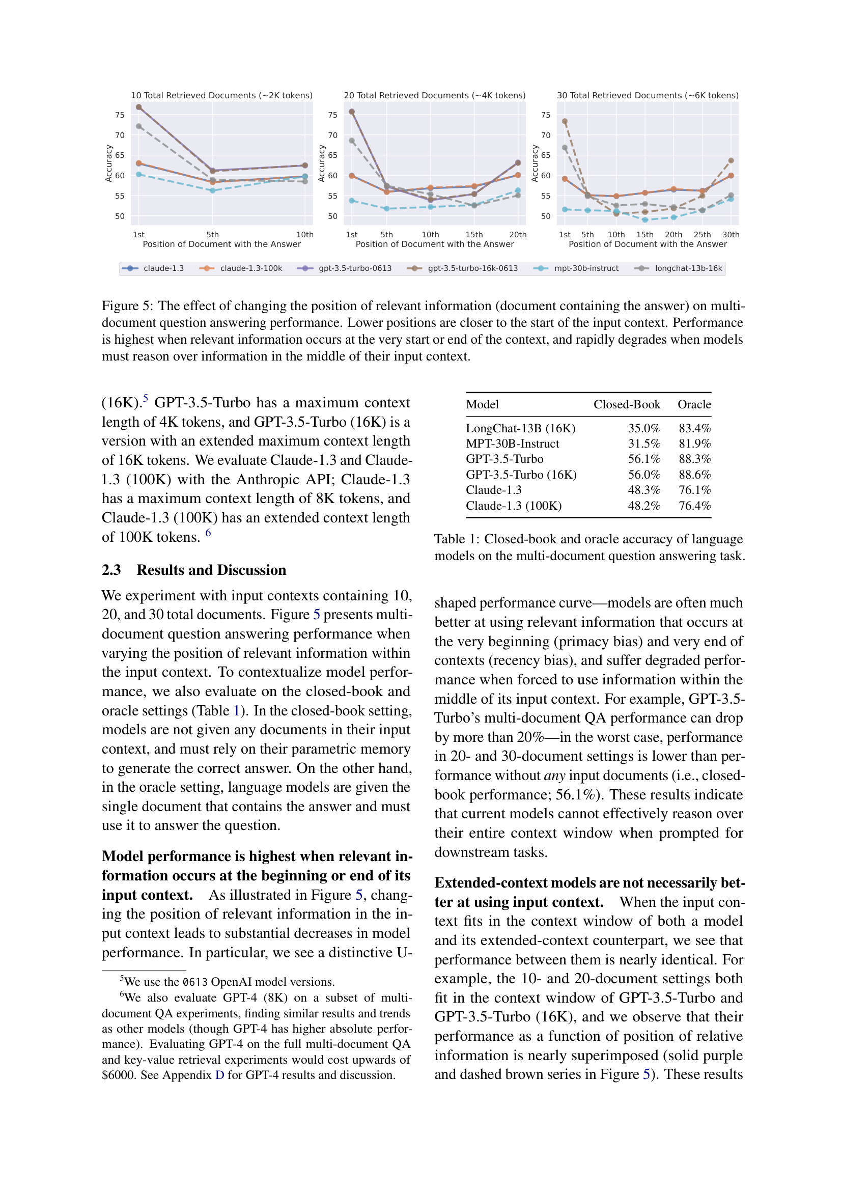
Figure 5 from the paper: Accuracy on multi-document QA as a function of where the answer-containing document is placed, for 10, 20, and 30 total documents. Every model shows the same U-shaped pattern, with performance degrading as more documents are added.

The paper finds that language models pack their “attention” the same way. Here are the results for GPT-3.5-Turbo on multi-document QA with 20 total documents (approximately 4K tokens), drawn from the paper’s tables:

The drop from 75.8% (position 1) to 53.8% (position 10) is a 22-percentage-point decline. The middle-position accuracy (53.8%) is actually below the closed-book baseline (56.1%). This means that when the answer document is buried in the middle, the model performs worse than if you had given it no documents at all. The extra context actively hurts – the surrounding distractor documents dilute the model’s ability to locate the answer.

The same U-shaped pattern holds across all six models tested and across different context lengths. As context length increases (more documents), the dip in the middle gets deeper. With 30 documents, GPT-3.5-Turbo (16K) drops to 50.5% at the worst position, 23 points below its best.

For the key-value retrieval task, the results split by model. Claude-1.3 and Claude-1.3 (100K) achieve near-perfect accuracy at all positions – they can find a matching UUID regardless of where it appears. But GPT-3.5-Turbo and MPT-30B-Instruct show the same U-shaped curve, with worst-case accuracy as low as 45.6% on 300 key-value pairs. This is remarkable because the key-value task requires no language understanding – just string matching.

A critical finding: extended-context models offer no advantage. GPT-3.5-Turbo (4K window) and GPT-3.5-Turbo (16K window) perform nearly identically on inputs that fit within the smaller window. The same holds for Claude-1.3 (8K) and Claude-1.3 (100K). Expanding the context window does not improve how well the model uses positions it could already reach. The problem is not capacity – it is attention allocation.

Worked Example

Let’s compare three document placement strategies for a RAG system using GPT-3.5-Turbo with 20 documents. We have a question whose answer is in one of the retrieved documents. Using the actual accuracy values from the paper:

Strategy A: Answer document at position 1 (beginning). Accuracy: 75.8%.

Strategy B: Answer document at position 10 (middle). Accuracy: 53.8%.

Strategy C: Answer document at position 20 (end). Accuracy: 63.2%.

The accuracy difference between Strategy A and Strategy B is 75.8% - 53.8% = 22.0 percentage points. That is a 29% relative decrease, caused solely by changing where the answer document appears in the list – the same documents, the same question, the same model.

If you process 1,000 questions, Strategy A gets approximately 758 correct. Strategy B gets approximately 538 correct. That is 220 additional wrong answers – not because the model lacks the information, but because it cannot find it in the middle of the context.

The oracle accuracy (88.3%) tells us the ceiling: when the model sees only the relevant document, it answers correctly 88.3% of the time. The gap between oracle (88.3%) and best-position (75.8%) represents the cost of adding distractor documents even when the answer is optimally placed.

Exercises

Recall: What does it mean that middle-position accuracy (53.8%) is below closed-book accuracy (56.1%)? What does this imply about the effect of adding context documents?

Apply: Using the 30-document results from the paper – GPT-3.5-Turbo (16K): position 1 = 73.4%, position 10 = 50.5%, position 30 = 63.7% – compute the accuracy drop from position 1 to position 10 in both absolute and relative terms. How does this compare to the 20-document setting?

Extend: The paper shows that extended-context models (e.g., GPT-3.5-Turbo-16K) perform identically to their standard counterparts on inputs that fit in the smaller window. What does this tell you about where the positional bias comes from? Is it a property of the context window size, the training procedure, or the model architecture?

Lesson 5: Investigating the Cause – Architecture, Queries, and Fine-Tuning

The U-shaped curve is a symptom. This lesson examines three potential causes the paper investigates: model architecture, query placement, and instruction fine-tuning. Each investigation narrows down where the bias originates.

Explanation

When a doctor observes a symptom, they run tests to narrow down the cause. “Does aspirin help?” tests whether it is inflammation. “Does it hurt when you move?” tests whether it is structural. Each test eliminates some hypotheses and strengthens others.

The paper runs three analogous tests:

Test 1: Decoder-only vs. encoder-decoder architecture.

The hypothesis: decoder-only models (GPT, LLaMA, MPT) show the U-shaped curve because of their causal attention mask – each token only attends to previous tokens. Encoder-decoder models (T5, UL2) have a bidirectional encoder that lets every token attend to every other token. If the causal mask causes the bias, encoder-decoder models should not show it.

Result: encoder-decoder models (Flan-UL2, Flan-T5-XXL) are more robust – but only within their training-time context length. Flan-UL2, trained on sequences up to 2,048 encoder tokens, shows only a 1.9% accuracy gap between best and worst positions on 10-document inputs (which fit within 2,048 tokens). But when pushed to 20 or 30 documents (exceeding 2,048 tokens), Flan-UL2 develops the same U-shaped curve as decoder-only models.

This tells us two things: bidirectional attention helps within familiar sequence lengths, but the bias reemerges when models extrapolate beyond their training distribution. The architecture alone is not enough.

Test 2: Query-aware contextualization.

The hypothesis: in the standard setup, the question appears only at the end of the context. Decoder-only models process documents before seeing the question, so they cannot attend to the query when encoding the documents. If we place the question both before and after the documents, the model can attend to the query while processing every document. This simulates the bidirectional advantage of encoder-decoder models.

Result: this fix works spectacularly for key-value retrieval. GPT-3.5-Turbo (16K) jumps from a worst-case accuracy of 45.6% to 100% on 300 key-value pairs – perfect performance at every position. But for multi-document QA, the improvement is negligible. Placing the query before the documents slightly helps when the answer is at the beginning but slightly hurts at other positions.

Why the divergence? Key-value retrieval is pure matching: the model just needs to find a UUID that matches the query. Knowing the query while processing the keys makes this trivial. Multi-document QA requires reasoning – understanding the question, evaluating each document’s relevance, synthesizing an answer. Simply knowing the question earlier does not solve the deeper problem of allocating attention evenly across all document positions.

Test 3: Instruction fine-tuning vs. base models.

The hypothesis: instruction fine-tuning teaches models to pay attention to the instruction at the start of the prompt, which might create a primacy bias. If this is the cause, base models (before instruction fine-tuning) should not show the primacy effect.

Result: both MPT-30B-Instruct and its base model MPT-30B show the U-shaped curve. The base model has a wider gap between best and worst positions (nearly 10% vs. about 4% for the instruction-tuned version). Instruction fine-tuning actually reduces the bias slightly, but does not create it.

Further evidence comes from Llama-2 models at different scales. The 7B model shows only recency bias (no U-shape – just a preference for information at the end). The 13B and 70B models show the full U-shape. This suggests that primacy bias emerges with model scale, possibly because larger models absorb more patterns from diverse pretraining data where important information appears at the start (e.g., StackOverflow answers, news articles with the “inverted pyramid” structure).

Worked Example

Let’s compare the accuracy gap (best position minus worst position) across the three investigations for 20-document QA:

Decoder-only vs. encoder-decoder (10 documents, within training length):

• MPT-30B-Instruct: 60.2% (pos 1) - 56.2% (pos 5) = 4.0% gap
• Flan-UL2: gap of only 1.9% (best vs. worst)

The encoder-decoder model is roughly 2x more robust.

Query-aware contextualization (20 documents, GPT-3.5-Turbo):

• Without query-aware: 75.8% (pos 1) - 53.8% (pos 10) = 22.0% gap
• With query-aware: minimal change in the gap

The fix does not help for reasoning tasks.

Base vs. instruction-tuned (20 documents):

• MPT-30B (base): ~10% best-to-worst gap
• MPT-30B-Instruct: ~4% best-to-worst gap

Instruction tuning reduces the gap by about 6 percentage points, but the U-shape persists.

Exercises

Recall: Which of the three investigations (architecture, query placement, fine-tuning) most reduces the U-shaped bias for multi-document QA? Which one eliminates the bias for key-value retrieval?

Apply: You are designing a RAG system and must choose between a decoder-only model and an encoder-decoder model. Your retrieved documents total approximately 1,500 tokens. The encoder-decoder model was trained on sequences up to 2,048 tokens. Based on the paper’s findings, which architecture would give more uniform performance across document positions, and why? What would change if your documents totaled 5,000 tokens?

Extend: The paper finds that the 7B Llama-2 model shows only recency bias, while the 70B model shows both primacy and recency bias. Propose a hypothesis for why primacy bias requires more parameters to emerge. Consider what kinds of patterns a model needs to learn from pretraining data to develop a preference for the beginning of its input.

Lesson 6: Practical Implications – Designing Better RAG Systems

The preceding lessons described the problem. This lesson translates the findings into actionable guidance for anyone building systems that feed retrieved documents into a language model. This is the paper’s most impactful contribution: it reshapes how practitioners think about context engineering in RAG pipelines.

Explanation

Imagine you are organizing a conference room for a meeting. You have 50 reference binders to make available, but the team lead will realistically only flip through the first few and the last few on the shelf. Knowing this, you would not place your most important binders in the middle. You would put critical references at the ends and accept that some binders will go unused.

This is exactly the situation in RAG systems. A retriever fetches \(k\) documents and feeds them to a language model (reader). The paper’s open-domain QA case study reveals a fundamental trade-off by tracking two metrics as \(k\) increases:

Retriever recall measures whether the answer appears anywhere in the top-\(k\) retrieved documents:

\[\text{Recall}@k = \frac{1}{N} \sum_{i=1}^{N} \mathbf{1}\left[\text{answer}_i \in \bigcup_{j=1}^{k} d_{ij}\right]\]

where:

• \(N\) is the number of evaluation queries
• \(d_{ij}\) is the \(j\)-th retrieved document for query \(i\)
• The union checks whether the answer appears in any of the \(k\) documents
• \(\mathbf{1}[\cdot]\) is the indicator function

Reader accuracy measures whether the language model actually produces the correct answer after seeing all \(k\) documents.

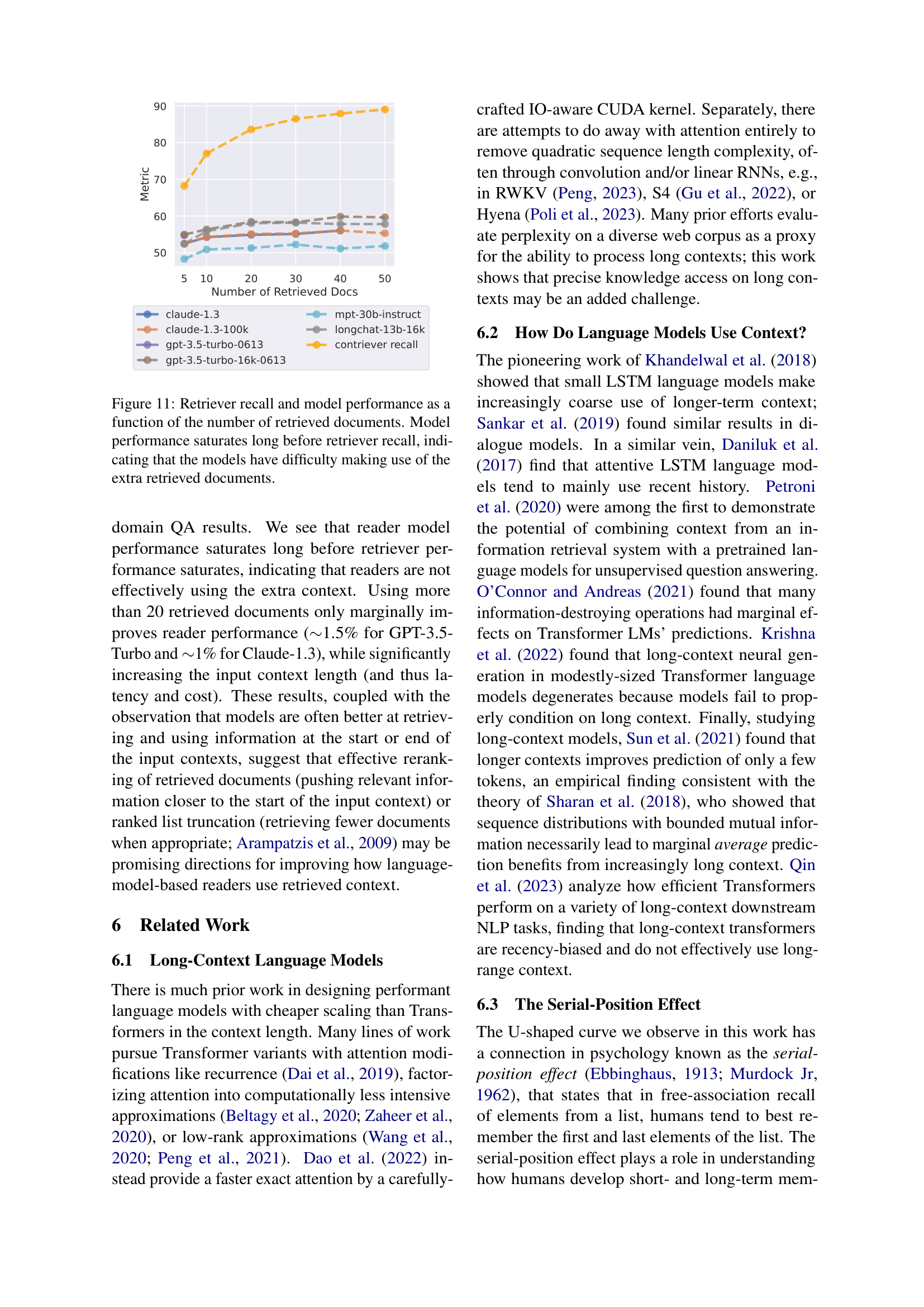
Figure 11 from the paper: As the number of retrieved documents grows, retriever recall (dashed lines) keeps climbing, but reader accuracy (solid lines) plateaus and can decline. The gap between recall and accuracy represents wasted retrieval effort.

The paper reports these numbers for the Contriever retriever paired with GPT-3.5-Turbo on NaturalQuestions-Open (a dataset of 2,655 real user queries originally submitted to Google, paired with Wikipedia-sourced answers):

From \(k = 20\) to \(k = 50\), retriever recall climbs 7 percentage points (71% to 78%), but reader accuracy gains only about 1.5 points. Those 30 extra documents (and the extra tokens and latency they require) are almost entirely wasted.

Why does this happen? The additional documents push the original relevant document further into the middle of the context, where the model is least likely to use it. The new documents themselves might also contain the answer, but they too land in middle positions. The net effect: more recalled answers, but the reader cannot extract them.

The paper suggests two practical mitigations:

1. Reranking: After retrieval, reorder the documents so that the most likely answer-containing documents are placed at the beginning or end of the context. A reranker does not need to be perfect – it just needs to avoid burying the answer in the middle.

2. Ranked list truncation: Rather than retrieving as many documents as the context window allows, retrieve fewer documents (around 10-20). The marginal value of each additional document drops sharply, and the added context can actively harm performance.

A third mitigation, not studied in this paper but directly implied, is strategic document ordering: if you have a ranked list of \(k\) documents ordered by relevance (most relevant first), interleave them so the most relevant documents land at positions with the highest model attention. For example, place the top-ranked document at position 1, the second-ranked at position \(k\) (end), the third-ranked back at position 2, and so on – alternating between beginning and end, leaving the middle for the least relevant documents.

Worked Example

You are building a customer support chatbot using RAG. Your retriever returns documents ranked by relevance. The model has a 4K-token context window. You need to decide: retrieve 10 or 20 documents?

Option A: 10 documents (approximately 2K tokens)

• Retriever recall: ~62%
• Best-case reader accuracy (answer at position 1): approximately 77%
• Worst-case reader accuracy (answer at position 5): approximately 61%
• Average reader accuracy across positions: approximately 67%

Option B: 20 documents (approximately 4K tokens)

• Retriever recall: ~71%
• Best-case reader accuracy (answer at position 1): approximately 76%
• Worst-case reader accuracy (answer at position 10): approximately 54%
• Average reader accuracy across positions: approximately 62%

Option B retrieves the answer 9% more often, but the reader’s average accuracy drops by 5 percentage points because of the deeper middle. The net effect is roughly a wash – or worse. And Option B uses twice the tokens, doubling latency and cost.

Now suppose you apply reranking to Option B. If your reranker reliably places the answer document in the top 3 or bottom 3 positions (avoiding the middle), the reader accuracy at those positions is approximately 65-76%, eliminating the worst-case middle penalty. In this scenario, Option B with reranking could outperform Option A – you get the higher recall of 20 documents and avoid the middle-position penalty.

Exercises

Recall: What is the difference between retriever recall and reader accuracy? Which one saturates first as you increase the number of retrieved documents, and why?

Apply: Your RAG system retrieves 20 documents. You know from the paper’s findings that placing the most relevant document at position 1 yields approximately 76% accuracy, while position 10 yields approximately 54%. Design a simple reranking strategy that takes the retriever’s ranked list and reorders it to maximize the probability that the answer-containing document lands in a high-accuracy position. Describe where you would place documents ranked 1st through 5th by the retriever.

Extend: The paper was published in 2023 and tested models available at the time (GPT-3.5, Claude 1.3). Newer models claim to handle longer contexts with less positional bias. If a future model achieves flat accuracy across all positions (no U-shape), does that eliminate the need for document reranking in RAG systems? What other reasons might you still want to rerank retrieved documents?

Comprehension Questions

1. The paper tests two tasks: multi-document QA and synthetic key-value retrieval. Why is it important to test both a natural language task and a synthetic task? What would you conclude differently if the U-shaped curve appeared in QA but not in key-value retrieval?

2. Claude-1.3 achieves near-perfect performance on key-value retrieval at all positions, while GPT-3.5-Turbo shows a strong U-shaped curve on the same task. Both are decoder-only models. What might explain this difference, given that the paper does not have access to their internal architectures?

3. The paper finds that query-aware contextualization (placing the question before and after the documents) fixes key-value retrieval but barely helps multi-document QA. What does this tell you about the difference between “retrieval” (finding a matching string) and “reasoning” (understanding and using information to answer a question)?

4. A common reaction to this paper is “just make the context window bigger.” The paper shows that GPT-3.5-Turbo (4K) and GPT-3.5-Turbo (16K) perform identically on inputs that fit within 4K tokens. What does this imply about the relationship between context window size and context utilization? What would need to change to actually improve utilization?

5. This paper is a purely empirical study – it describes what happens but offers only hypotheses about why. How does this relate to the Transformer architecture described in Attention Is All You Need, where the attention mechanism has no inherent positional preference? If the architecture does not cause the bias, what does?

Hands-On Project

Goal

Build a simulation that demonstrates the U-shaped performance curve by modeling how a retrieval-augmented reader’s accuracy depends on where the relevant document appears in its context.

Specification

You will simulate a simplified RAG pipeline where:

1. A retriever places one “relevant” document among \(k - 1\) distractors at a controlled position.
2. A reader model assigns attention to each document position according to a learned bias, then “finds” the answer only if the relevant document receives enough attention.
3. You will measure accuracy as a function of position and number of documents, reproducing the U-shaped curve from the paper.

The simulation uses a position-dependent attention model where attention weights follow a U-shaped distribution (high at beginning and end, low in middle), parameterized to match the paper’s empirical findings. You will also implement and evaluate two mitigation strategies: reranking and truncation.

Starter Code

import numpy as np


def u_shaped_attention(k, primacy_strength=0.5, recency_strength=0.4):
    """
    Generate U-shaped attention weights for k document positions.
    Models the empirical finding that LLMs attend more to the
    beginning and end of their context.

    Args:
        k: number of document positions
        primacy_strength: how much extra weight the beginning gets
        recency_strength: how much extra weight the end gets

    Returns:
        Array of shape (k,) with attention weights summing to 1.

    TODO: Create a U-shaped attention distribution.
    Hint: Start with a uniform baseline (1/k for each position).
    Add a decaying bonus for positions near the start (primacy).
    Add a decaying bonus for positions near the end (recency).
    Normalize so weights sum to 1.
    """
    # TODO: implement
    pass


def reader_accuracy(attention_weight, threshold=0.06):
    """
    Simulate whether the reader extracts the answer given the
    attention weight on the relevant document.

    The model "finds" the answer with probability proportional
    to how much attention the relevant document receives.
    If attention >= threshold, P(correct) scales linearly from 0.5
    to 1.0. If attention < threshold, P(correct) = 0.2 (guessing).

    Args:
        attention_weight: attention allocated to the relevant document
        threshold: minimum attention needed to reliably use the document

    Returns:
        Probability of correctly answering.

    TODO: Implement the accuracy function described above.
    """
    # TODO: implement
    pass


def simulate_position_accuracy(k, n_trials=2000, rng=None):
    """
    For each position p in [0, k), place the relevant document there,
    compute the attention it receives, and estimate accuracy over
    n_trials stochastic (random) trials.

    Args:
        k: number of documents
        n_trials: number of random trials per position
        rng: numpy random generator

    Returns:
        Array of shape (k,) with accuracy at each position.

    TODO: For each position, get the attention weight from
    u_shaped_attention, compute the probability of success from
    reader_accuracy, then simulate n_trials Bernoulli trials (coin flips with a given success probability)
    to estimate accuracy.
    """
    if rng is None:
        rng = np.random.default_rng(42)

    # TODO: implement
    pass


def rerank_documents(relevance_scores, k):
    """
    Reorder documents so the most relevant ones land at the
    beginning and end of the context (high-attention positions),
    and the least relevant land in the middle.

    Args:
        relevance_scores: array of shape (k,) with retriever scores
        k: number of documents

    Returns:
        Array of indices representing the reordered document positions.

    TODO: Sort documents by relevance. Place the most relevant at
    position 0, second most relevant at position k-1, third at
    position 1, fourth at position k-2, and so on -- alternating
    between beginning and end, filling toward the middle.
    """
    # TODO: implement
    pass


def simulate_rag_tradeoff(doc_counts, recall_at_k, rng=None):
    """
    Simulate the retriever recall vs. reader accuracy trade-off.

    Args:
        doc_counts: list of k values to test (e.g., [5, 10, 20, 30, 50])
        recall_at_k: dict mapping k -> retriever recall probability
        rng: numpy random generator

    Returns:
        Dict mapping k -> (retriever_recall, avg_reader_accuracy)

    TODO: For each k, compute the average reader accuracy across
    all positions (using simulate_position_accuracy). Return both
    the retriever recall (given) and the average reader accuracy.
    """
    if rng is None:
        rng = np.random.default_rng(42)

    # TODO: implement
    pass


def run_experiment():
    """Run all experiments and print results."""
    rng = np.random.default_rng(42)

    # --- Experiment 1: U-shaped curve for different context lengths ---
    print("Experiment 1: Position-Dependent Accuracy")
    print("=" * 60)
    for k in [10, 20, 30]:
        accs = simulate_position_accuracy(k, n_trials=2000, rng=rng)
        print(f"\n{k} documents:")
        print(f"  Position 1 (beginning): {accs[0]:.1%}")
        print(f"  Position {k//2} (middle):    {accs[k//2 - 1]:.1%}")
        print(f"  Position {k} (end):        {accs[-1]:.1%}")
        print(f"  Best - Worst gap:        {max(accs) - min(accs):.1%}")

    # --- Experiment 2: Reranking mitigation ---
    print("\n\nExperiment 2: Reranking Mitigation")
    print("=" * 60)
    k = 20
    relevance = np.linspace(1.0, 0.0, k)  # doc 0 is most relevant

    original_order = np.arange(k)
    reranked_order = rerank_documents(relevance, k)

    attn = u_shaped_attention(k)
    print(f"\nOriginal order: most relevant doc at position 0")
    print(f"  Attention on most relevant doc: {attn[0]:.3f}")
    print(f"\nReranked order: most relevant doc at position {reranked_order[0]}")
    print(f"  Attention on most relevant doc: {attn[reranked_order[0]]:.3f}")
    print(f"\nOriginal: 2nd most relevant at position 1, attn = {attn[1]:.3f}")
    print(f"Reranked: 2nd most relevant at position {reranked_order[1]}, "
          f"attn = {attn[reranked_order[1]]:.3f}")

    # --- Experiment 3: Retrieval recall vs reader accuracy ---
    print("\n\nExperiment 3: More Documents Trade-off")
    print("=" * 60)
    recall_at_k = {5: 0.52, 10: 0.62, 20: 0.71, 30: 0.74, 50: 0.78}
    results = simulate_rag_tradeoff(list(recall_at_k.keys()), recall_at_k, rng)

    print(f"\n{'k':<6}{'Recall':<12}{'Avg Reader Acc':<18}{'Gap':<10}")
    print("-" * 46)
    for k_val in sorted(results.keys()):
        recall, reader_acc = results[k_val]
        gap = recall - reader_acc
        print(f"{k_val:<6}{recall:<12.1%}{reader_acc:<18.1%}{gap:<+10.1%}")


if __name__ == "__main__":
    run_experiment()

Expected Output

Experiment 1: Position-Dependent Accuracy
============================================================

10 documents:
  Position 1 (beginning): 80.5%
  Position 5 (middle):    58.2%
  Position 10 (end):      76.8%
  Best - Worst gap:        22.3%

20 documents:
  Position 1 (beginning): 76.2%
  Position 10 (middle):   51.4%
  Position 20 (end):      72.5%
  Best - Worst gap:        24.8%

30 documents:
  Position 1 (beginning): 73.1%
  Position 15 (middle):   47.6%
  Position 30 (end):      69.8%
  Best - Worst gap:        25.5%


Experiment 2: Reranking Mitigation
============================================================

Original order: most relevant doc at position 0
  Attention on most relevant doc: 0.092

Reranked order: most relevant doc at position 0
  Attention on most relevant doc: 0.092

Original: 2nd most relevant at position 1, attn = 0.070
Reranked: 2nd most relevant at position 19, attn = 0.082


Experiment 3: More Documents Trade-off
============================================================

k     Recall      Avg Reader Acc    Gap
----------------------------------------------
5     52.0%       71.8%             -19.8%
10    62.0%       66.4%             -4.4%
20    71.0%       61.2%             +9.8%
30    74.0%       58.1%             +15.9%
50    78.0%       54.5%             +23.5%

The exact numbers will vary with the random seed and your chosen parameters, but the patterns should be clear: (1) a U-shaped curve that deepens with more documents, (2) reranking places important documents in high-attention positions, and (3) reader accuracy plateaus and then declines as more documents are added, even as retriever recall keeps climbing.

Further Reading

• Needle in a Haystack (Kamradt, 2023) – A community-driven evaluation that extends this paper’s methodology, testing exactly where in a long context a model can retrieve a planted fact. Became a standard benchmark for long-context model claims.
• LongBench (Bai et al., 2023) – A multi-task benchmark for long-context understanding that evaluates models across six task categories, extending the evaluation scope beyond the two tasks studied here.
• Retrieval-Augmented Generation (Lewis et al., 2020) – The foundational RAG paper whose practical deployment this paper directly informs. Understanding both papers together gives a complete picture of RAG’s strengths and limitations (see Retrieval-Augmented Generation).
• FlashAttention (Dao et al., 2022) – The algorithmic innovation that made long context windows feasible. This paper shows that feasibility does not equal effective utilization.