By the end of this course, you will be able to:
Imagine a restaurant kitchen with one master chef who knows every recipe. Now imagine that for each new customer who orders a different dish, you must clone the entire chef – their years of training, all their knowledge – just to change how they plate the food. That is what full fine-tuning does: it copies every single parameter of a large model to change the behavior on each new task.
In transfer learning, you take a model pre-trained on a large dataset and adapt it to a new, usually smaller, task. By 2019, the standard approach was full fine-tuning: copy all the weights of a model like BERT, then update every weight on the new task’s training data. BERT-Large has 330 million parameters. If you fine-tune it for 9 different tasks (the GLUE benchmark – a collection of nine natural language understanding tasks used to evaluate general-purpose language representations), you need 9 separate copies: \(9 \times 330\text{M} = 2.97\) billion parameters in total.
Formally, consider a pre-trained network \(\phi_w(x)\) with parameters \(w\). Fine-tuning updates \(w\) for each task, producing task-specific parameter sets \(w_1, w_2, \ldots, w_N\). The total storage is:
\[\text{Total parameters} = N \times |w|\]
where \(N\) is the number of tasks and \(|w|\) is the number of parameters in the pre-trained model.
There is an alternative: feature-based transfer. Instead of changing the pre-trained weights, you freeze them and train a new, small function \(\chi_v\) on top:
\[\chi_v(\phi_w(x))\]
where only \(v\) is trained and \(w\) stays frozen. This is parameter efficient – you only store \(|w| + N \times |v|\) total parameters – but it performs worse because the pre-trained features cannot adapt to the task at all.
The paper frames the problem crisply: feature-based transfer is cheap but weak, fine-tuning is strong but expensive. The field needs a method that gets fine-tuning-level performance at feature-extraction-level cost.
There is a third practical problem beyond storage: catastrophic forgetting. When you fine-tune a model on Task A and then fine-tune the same copy on Task B, the model loses its ability to do Task A. Each task’s fine-tuning destructively overwrites the shared weights. You cannot incrementally add new tasks – each one starts from scratch.
Suppose you run a cloud service with BERT-Base (110M parameters) and need to serve 17 text classification tasks. Calculate the total parameter budget under each strategy:
Full fine-tuning: each task gets its own copy of all 110M parameters.
Feature-based transfer: freeze BERT-Base and train a linear classifier per task. A classifier for a task with \(C = 4\) classes on BERT-Base’s 768-dimensional output has \(768 \times 4 + 4 = 3{,}076\) parameters.
Adapter tuning (what this paper proposes): freeze BERT-Base, add small adapter modules per task. With adapters using 1.14% of parameters per task:
The jump from \(17\times\) (fine-tuning) to \(1.19\times\) (adapters) while losing less than 0.5% accuracy is the paper’s central result.
Recall: What are the two practical problems with full fine-tuning when serving many tasks? Name both.
Apply: You have a BERT-Large model (330M parameters) and need to serve 50 tasks. How many total parameters does full fine-tuning require? How about adapter tuning at 3.6% parameters per task? Express both as multiples of the base model size.
Extend: Suppose a company serves 1,000 customer-specific models. At what point does the difference between fine-tuning and adapter tuning start to matter for a budget – when models are 100M parameters? 1B? 100B? What factors beyond parameter count matter (think about GPU memory, loading time, and serving infrastructure)?
A bottleneck in engineering is a narrow passage that restricts flow. In a factory, you might funnel thousands of parts through a single inspection point, then fan them back out to their respective assembly lines. The bottleneck forces everything through a compact representation. In neural networks, a bottleneck layer compresses a high-dimensional representation into a much smaller one, applies a transformation, then expands it back. This compression forces the network to learn a compact encoding of what matters.
The adapter module is a two-layer neural network with a bottleneck shape. It takes an input vector \(h\) of dimension \(d\) (the hidden size of the Transformer – 768 for BERT-Base), squeezes it down to a much smaller dimension \(m\), and then expands it back to \(d\).
The down-projection compresses \(d\) dimensions to \(m\) dimensions:
\[z = h W_{\text{down}}\]
where \(h \in \mathbb{R}^d\) is the input, \(W_{\text{down}} \in \mathbb{R}^{d \times m}\) is the down-projection weight matrix, and \(z \in \mathbb{R}^m\) is the compressed representation.
A nonlinear activation function is applied element-wise:
\[a = f(z)\]
where \(f\) is a nonlinearity. The paper uses ReLU (Rectified Linear Unit), which simply sets all negative values to zero: \(f(x) = \max(0, x)\). Without this nonlinearity, the two projections would collapse into a single linear transformation and the adapter could not learn nonlinear task-specific features.
The up-projection expands back from \(m\) to \(d\) dimensions:
\[\hat{h} = a W_{\text{up}}\]
where \(W_{\text{up}} \in \mathbb{R}^{m \times d}\) is the up-projection weight matrix and \(\hat{h} \in \mathbb{R}^d\) is the output.
The parameter count for one adapter (including bias terms) is:
\[P_{\text{adapter}} = 2md + d + m\]
where \(2md\) accounts for the two weight matrices (\(d \times m\) down-projection and \(m \times d\) up-projection), \(m\) is the bias for the down-projection, and \(d\) is the bias for the up-projection.
The bottleneck dimension \(m\) controls the trade-off between capacity and efficiency. The paper tests values from 2 to 256. Setting \(m \ll d\) ensures the adapter is small relative to the main model.
Let \(d = 6\) (hidden dimension) and \(m = 2\) (bottleneck dimension). Our input vector is:
\[h = [0.5, -0.3, 0.8, 0.1, -0.6, 0.4]\]
Step 1: Down-projection. Multiply by \(W_{\text{down}}\) (a \(6 \times 2\) matrix) and add bias \(b_{\text{down}}\):
\[W_{\text{down}} = \begin{bmatrix} 0.2 & -0.1 \\ 0.3 & 0.4 \\ -0.1 & 0.2 \\ 0.5 & -0.3 \\ 0.1 & 0.6 \\ -0.2 & 0.1 \end{bmatrix}, \quad b_{\text{down}} = [0.0, 0.0]\]
\[z = h \cdot W_{\text{down}} + b_{\text{down}}\]
Computing each element:
So \(z = [-0.16, -0.36]\). We compressed from 6 dimensions to 2.
Step 2: ReLU. Apply \(f(x) = \max(0, x)\):
\[a = [\max(0, -0.16), \max(0, -0.36)] = [0.0, 0.0]\]
Both values are negative, so ReLU zeros them out.
Step 3: Up-projection. Multiply by \(W_{\text{up}}\) (a \(2 \times 6\) matrix) and add bias \(b_{\text{up}}\):
Since \(a = [0.0, 0.0]\), the result is simply the bias: \(\hat{h} = b_{\text{up}}\).
This illustrates an important point: when the adapter weights are small (or produce negative activations), the output of the adapter is near zero. This is exactly what happens at initialization.
Parameter count: \(2 \times 6 \times 2 + 6 + 2 = 24 + 8 = 32\) parameters for this toy adapter. For BERT-Base with \(d = 768\) and \(m = 64\): \(2 \times 768 \times 64 + 768 + 64 = 98{,}304 + 832 = 99{,}136\) parameters.
Recall: Why is a nonlinear activation function (like ReLU) necessary between the down-projection and up-projection? What would happen without it?
Apply: Calculate the parameter count for a single adapter module with \(d = 1024\) (BERT-Large) and \(m = 8\). Then calculate it for \(m = 256\). What is the ratio between them?
Extend: The bottleneck forces the adapter to learn a compressed representation in \(m\) dimensions. If your task is very simple (binary sentiment classification), would you expect a small or large \(m\) to suffice? What about a complex task with 157 classes? The paper’s results show adapter sizes of 8 to 256 across tasks – what does this range tell you about task complexity?
Think of a highway bypass. When a new stretch of road is under construction, traffic can still flow on the original highway. The new section carries no traffic initially – it starts “closed.” As construction finishes, traffic gradually shifts to use the new route. This is exactly what a skip connection does for an adapter: it lets the original signal pass through unmodified while the new adapter parameters start from near-zero, initially contributing nothing and gradually learning task-specific adjustments.
The complete adapter computation, including the internal skip connection, is:
\[h \leftarrow h + f(h W_{\text{down}}) W_{\text{up}}\]
where \(h \in \mathbb{R}^d\) is the input hidden representation, \(W_{\text{down}} \in \mathbb{R}^{d \times m}\) is the down-projection, \(W_{\text{up}} \in \mathbb{R}^{m \times d}\) is the up-projection, and \(f\) is the ReLU activation. The critical piece is the leading “\(h +\)” – the skip connection (also called a residual connection). The adapter’s output is added to its input, rather than replacing it.
This skip connection enables near-identity initialization. If the adapter weights \(W_{\text{down}}\) and \(W_{\text{up}}\) are initialized near zero, then \(f(h W_{\text{down}}) W_{\text{up}} \approx 0\), and the output is approximately:
\[h + 0 = h\]
The adapter acts as the identity function – it passes the input through unchanged. This means that when training begins, the modified network \(\psi_{w,v}(x)\) behaves almost identically to the original pre-trained network \(\phi_w(x)\):
\[\psi_{w,v_0}(x) \approx \phi_w(x)\]
This property is essential for two reasons:
Stable starting point. Training starts from a model that already works well on general language tasks. The adapter does not disrupt what the pre-trained model has learned. Gradients flow normally through the network because the initial configuration is a known-good state.
Graceful adaptation. As training progresses, the adapter weights grow from near-zero to task-specific values. The adapter gradually “turns on” – first making small corrections, then larger task-specific modifications. This is more stable than starting from random weights that immediately distort the pre-trained representations.
The paper initializes adapter weights by drawing from a zero-mean Gaussian with standard deviation \(10^{-2}\), truncated to two standard deviations. Their analysis shows that performance is stable for initialization scales below \(10^{-2}\), but degrades when the scale is too large – confirming that near-identity initialization matters.
Let \(d = 4\) and \(m = 2\), with input \(h = [1.0, 0.5, -0.8, 0.3]\).
Case 1: Near-zero initialization (standard deviation \(10^{-2}\)).
\[W_{\text{down}} = \begin{bmatrix} 0.005 & -0.008 \\ 0.012 & 0.003 \\ -0.007 & 0.011 \\ 0.009 & -0.006 \end{bmatrix}\]
Down-project (ignoring biases for clarity):
After ReLU: \(a = [0.0193, 0.0]\)
\[W_{\text{up}} = \begin{bmatrix} 0.003 & -0.01 & 0.007 & 0.002 \\ -0.006 & 0.004 & 0.009 & -0.005 \end{bmatrix}\]
Up-project: \(\hat{h} = [0.0193 \times 0.003, \; 0.0193 \times (-0.01), \; 0.0193 \times 0.007, \; 0.0193 \times 0.002]\) \(= [0.0001, -0.0002, 0.0001, 0.00004]\)
After skip connection: \(h_{\text{out}} = h + \hat{h} = [1.0001, 0.4998, -0.7999, 0.30004]\)
The output is almost identical to the input. The adapter changes the representation by less than 0.03%.
Case 2: Large initialization (standard deviation \(1.0\)).
If the weights were 100 times larger, the adapter output \(\hat{h}\) would be roughly 100 times larger too. Instead of a 0.03% perturbation, you would get a 3% perturbation – enough to destabilize a pre-trained model that expects its internal representations to stay within learned ranges.
Recall: What two properties of the adapter design enable the near-identity initialization? Name both.
Apply: An adapter with \(d = 768\) and \(m = 64\) has weights initialized from \(\mathcal{N}(0, 0.01^2)\). Estimate the magnitude of a typical adapter output element before the skip connection. (Hint: each output element is the dot product of a 64-dimensional vector of ReLU-activated values with a 64-dimensional column of \(W_{\text{up}}\). Both have entries on the order of \(0.01\).)
Extend: The paper found that initialization scales above \(10^{-2}\) hurt performance, especially on smaller datasets like CoLA. Why might smaller datasets be more sensitive to initialization scale? Think about the relationship between the amount of training data and the model’s ability to recover from a bad starting point.
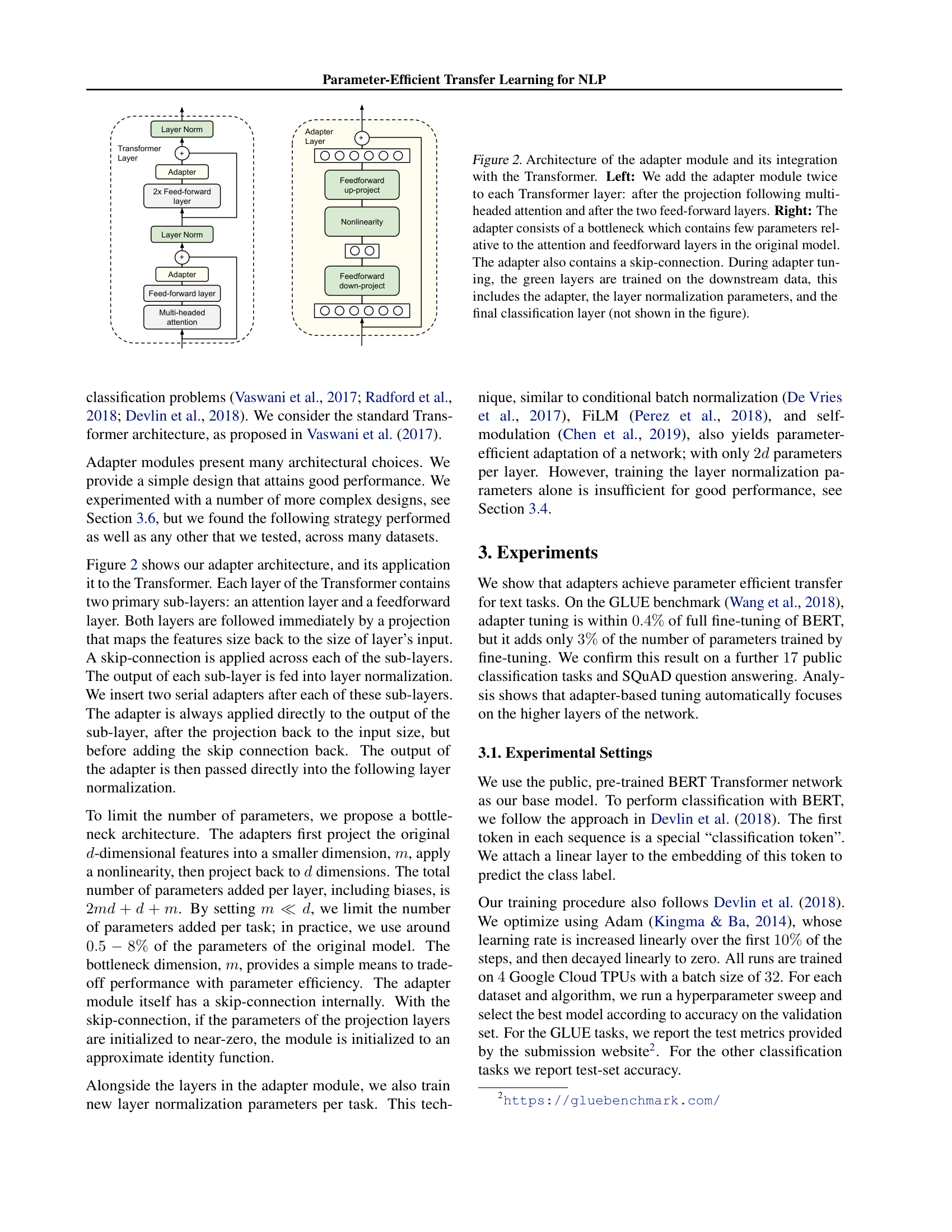
You know how adapters work in isolation. Now the question is: where do you insert them in the Transformer? A Transformer layer has two main sub-layers (attention and feedforward), each followed by a residual connection and layer normalization. The placement of adapters relative to these components determines what representations the adapters can modify and how training gradients flow.
Recall the standard Transformer layer structure (see Attention Is All You Need). Each layer has two sub-layers:
The paper inserts an adapter module at two points per layer:
In pseudocode, one Transformer layer with adapters looks like this:
# Sub-layer 1: Attention
attn_output = multi_head_attention(h)
attn_output = project(attn_output)
attn_output = adapter_1(attn_output)     # <-- adapter inserted here
h = layer_norm(h + attn_output)          # residual + layer norm

# Sub-layer 2: Feedforward
ff_output = feedforward(h)
ff_output = project(ff_output)
ff_output = adapter_2(ff_output)         # <-- adapter inserted here
h = layer_norm(h + ff_output)            # residual + layer norm
The adapter sits between the sub-layer’s output projection and the Transformer’s own residual connection. This placement means the adapter can modify what gets added to the residual stream without interfering with the residual connection itself. The adapter has its own internal skip connection (from Lesson 3), and the Transformer has its external skip connection. These are separate mechanisms – the adapter’s skip connection enables near-identity initialization, while the Transformer’s skip connection preserves information flow across layers.
During training, the adapter parameters and layer normalization parameters are updated. Everything else – all attention weights, feedforward weights, and embedding weights – stays frozen. The layer normalization parameters are re-trained because they are small (\(2d\) parameters per layer, compared to millions in the attention and feedforward weights) and adapting them helps the model adjust its internal statistics.
The paper’s ablation study (systematically removing or varying one component at a time to measure its contribution) reveals an asymmetry: adapters in the lower layers (layers 0-4 in BERT-Base’s 12 layers) contribute much less than adapters in the higher layers. Removing adapters from layers 0-4 barely affects accuracy on MNLI, while removing all adapters drops performance to the majority-class baseline. This aligns with a general finding in deep networks: lower layers learn generic features (syntax, word relationships) shared across tasks, while higher layers learn task-specific features (sentiment polarity, entailment relationships).
Consider a simplified 2-layer Transformer with \(d = 4\) and adapter bottleneck \(m = 2\). Count the trainable parameters for a single task.
Per-layer adapter parameters:
Per-layer layer normalization parameters:
Per-layer trainable total: \(44 + 16 = 60\) parameters
Whole model (2 layers): \(2 \times 60 = 120\) adapter and layer norm parameters
Now compare to the frozen parameters. Each layer has:
Frozen for 2 layers: \({\approx}384\) parameters. Trainable: 120 parameters. The ratio is \(120 / (384 + 120) \approx 24\%\). In our tiny toy example this seems high, but the ratio shrinks dramatically at real scale because the frozen attention and feedforward weights grow as \(O(d^2)\) while the adapter parameters grow as \(O(md)\) with \(m \ll d\).
At BERT-Base scale (\(d = 768\), 12 layers, \(m = 64\)):
Recall: At what two points within each Transformer layer does the paper insert adapter modules? What comes after the adapter in the processing pipeline?
Apply: BERT-Large has 24 layers and \(d = 1024\). Calculate the total number of adapter parameters when using bottleneck size \(m = 256\). Express as a percentage of BERT-Large’s 330M parameters.
Extend: The ablation study shows lower-layer adapters contribute less. The paper inserts adapters at every layer anyway. Can you think of a modified design that exploits this finding? What are the trade-offs of skipping adapters in lower layers versus keeping them?
We have all the components: the bottleneck architecture (Lesson 2), the near-identity initialization with skip connections (Lesson 3), and the placement strategy within the Transformer (Lesson 4). Now we assemble the full adapter tuning system and examine how it performs against the alternatives.
The adapter-based transfer approach can be summarized by a single equation. Given a pre-trained network \(\phi_w\) with parameters \(w\), we define a new network:
\[\psi_{w,v}(x) \quad \text{where} \quad \psi_{w,v_0}(x) \approx \phi_w(x)\]
where \(v\) represents all the adapter parameters and layer normalization parameters. During training, \(w\) is frozen and only \(v\) is updated using standard supervised learning on the downstream task.
The parameter efficiency constraint is:
\[|v| \ll |w| \implies \text{total for } N \text{ tasks} \approx |w| + N \cdot |v| \approx |w|\]
When \(|v|\) is small relative to \(|w|\), the total model size for \(N\) tasks stays close to \(|w|\) instead of growing as \(N \times |w|\).
Training procedure. The paper follows the standard BERT fine-tuning recipe: optimize with Adam (an adaptive learning rate optimizer that maintains per-parameter momentum and scaling), linearly warm up the learning rate for the first 10% of steps, then linearly decay to zero. The only adapter-specific hyperparameter is the bottleneck dimension \(m\), chosen from \(\{8, 64, 256\}\) per task. Due to training instability, the paper runs each configuration with 5 random seeds and selects the best on the validation set.
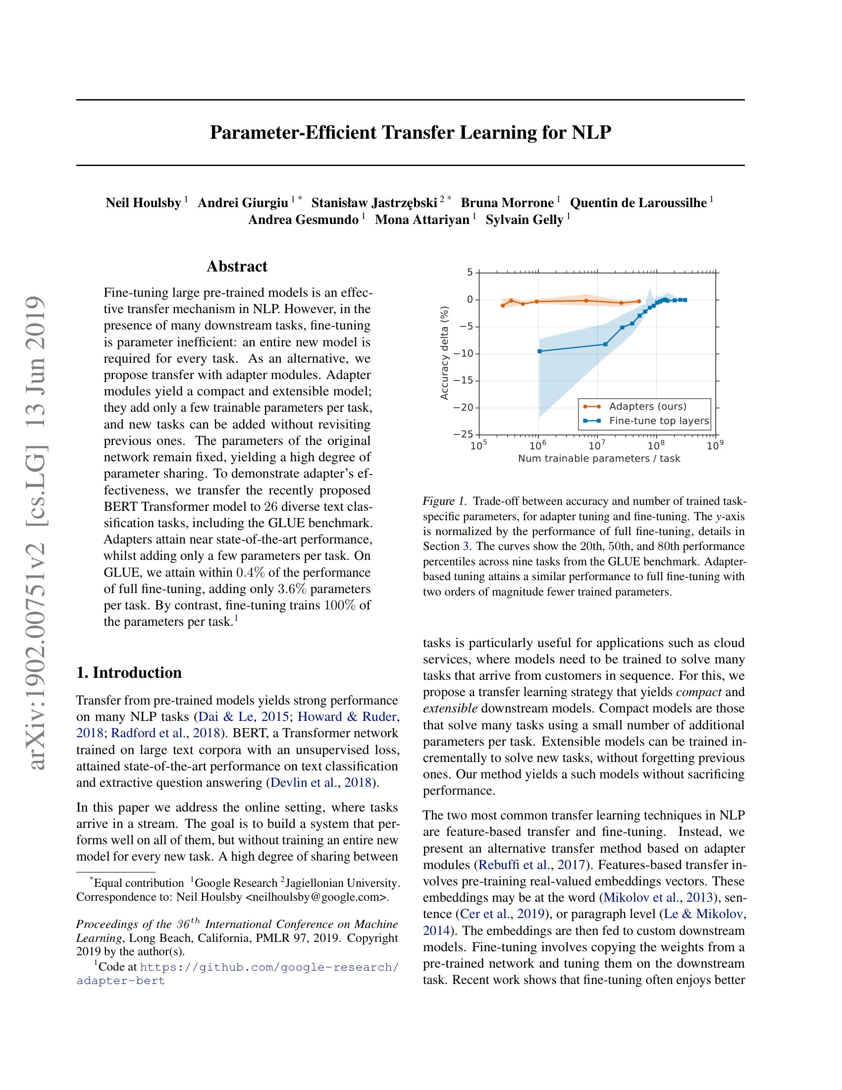
Results. On the GLUE benchmark (9 tasks, using BERT-Large):
| Method | Trained params/task | Total params (9 tasks) | Average Score |
|---|---|---|---|
| Full fine-tuning | 100% | 9.0x | 80.4 |
| Adapters (best \(m\) per task) | 3.6% | 1.3x | 80.0 |
| Adapters (fixed \(m = 64\)) | 2.1% | 1.2x | 79.6 |
Adapters reach within 0.4 points of full fine-tuning while requiring 7 times fewer total parameters. The optimal adapter size varies by task: MNLI (a large dataset with 393K examples) uses \(m = 256\), while RTE (a small dataset with 2.5K examples) uses \(m = 8\). Larger tasks benefit from more adapter capacity.
On 17 additional classification tasks using BERT-Base, adapters at 1.14% parameters per task achieve 73.3% average accuracy versus 73.7% for full fine-tuning – a gap of just 0.4% while reducing total model size from \(17\times\) to \(1.19\times\).
On SQuAD v1.1 (extractive question answering), adapters of size 64 (2% of parameters) score 90.4% F1 (the harmonic mean of precision and recall, balancing how many correct answers the model finds with how many of its answers are correct), compared to 90.7% for full fine-tuning. Even adapters of size 2 (0.1% of parameters) score 89.9% F1.
What the adapters learn. The ablation study removes adapters from continuous spans of layers and measures accuracy. Removing adapters from layers 0-4 barely affects MNLI accuracy. Removing all adapters drops performance to the majority-class baseline (37% on MNLI). No single adapter is critical – removing any one layer’s adapters drops accuracy by at most 2% – but their collective effect is large. The adapters have learned to distribute task-specific knowledge across many layers, with higher layers carrying more of the load.
Walk through the full adapter tuning pipeline for a single task: binary sentiment classification on a tiny dataset.
Setup:
Step 1: Initialize. Insert 4 adapter modules (2 per layer). Each adapter has \(2(2)(4) + 4 + 2 = 22\) parameters. Total adapter parameters: \(4 \times 22 = 88\). Initialize all adapter weights from \(\mathcal{N}(0, 0.01^2)\). The pre-trained Transformer weights are frozen.
Step 2: Forward pass (before training). The input flows through the Transformer. At each adapter, the near-zero weights produce a near-zero output. The skip connection passes the input through unchanged. The model produces the same output as the original pre-trained model – no task-specific behavior yet.
Step 3: Compute loss. The classification head (a linear layer mapping from \(d = 4\) to 2 classes) produces logits (raw unnormalized scores before conversion to probabilities). Suppose the model outputs \([0.2, -0.1]\) for classes [positive, negative]. The true label is “positive” (class 0). The cross-entropy loss (a loss function that measures how far the model’s predicted probability distribution is from the true label, reaching zero when the model assigns probability 1.0 to the correct class) is:
\[L = -\log\left(\frac{e^{0.2}}{e^{0.2} + e^{-0.1}}\right) = -\log\left(\frac{1.221}{1.221 + 0.905}\right) = -\log(0.574) = 0.555\]
Step 4: Backward pass. Gradients flow through the classification head, through the adapters, and through the Transformer – but only the adapter weights, layer normalization parameters, and classification head weights are updated. The pre-trained Transformer weights receive gradients but those gradients are discarded (weights frozen).
Step 5: After training. After many steps of gradient updates, the adapter weights have grown from near-zero to task-specific values. The adapters in higher layers have learned to emphasize features relevant to sentiment. The model now outputs high confidence for the correct sentiment class. The pre-trained weights remain exactly as they were.
Step 6: Add another task. To serve a second task (topic classification), create a new set of 88 adapter parameters. The 2-layer Transformer is shared. Total parameter overhead for the second task: 88 parameters (not a full copy of the Transformer).
Recall: What three categories of parameters are updated during adapter tuning? What stays frozen?
Apply: You deploy BERT-Base (110M parameters) with adapters (\(m = 64\), roughly 2.4M adapter parameters per task) to serve 100 tasks. Calculate the total parameters for: (a) full fine-tuning, (b) adapter tuning. What is the storage savings in gigabytes, assuming 4 bytes per parameter (float32)?
Extend: The paper reports that on SQuAD, adapters of size 2 (0.1% of parameters) still achieve 89.9% F1 versus 90.7% for full fine-tuning. Why might extractive question answering need so few task-specific parameters compared to tasks like CoLA (grammatical acceptability)? Think about what the pre-trained model already knows versus what each task demands.
Adapter tuning achieves comparable accuracy to full fine-tuning while training far fewer parameters. Where does the task-specific knowledge actually live? Is it only in the adapter weights, or does the frozen model contribute task-relevant computation too?
The paper initializes adapter weights from a truncated Gaussian with standard deviation \(10^{-2}\). Why not initialize to exactly zero? What would go wrong during training if all adapter weights started at precisely zero? (Hint: think about what happens to the gradients when all neurons compute the same function.)
Compare the parameter efficiency of three approaches: (a) fine-tuning only the top \(k\) layers, (b) adapter tuning, and (c) feature-based transfer. For a fixed parameter budget of 2% of the base model, which approach gives the best accuracy and why?
The paper only evaluates on classification and span extraction tasks. What challenges might adapter tuning face on generation tasks (text summarization, translation, open-ended dialogue)? Would you expect the adapter size needed to be larger or smaller for generation?
Adapter modules add serial computation to each layer. An alternative approach could modify the existing weight matrices in parallel instead. What are the practical implications of this difference for inference latency? Which approach would be faster at serving time and why?
Build a minimal adapter module and demonstrate that it starts as a near-identity function, can be trained to modify a frozen network’s behavior, and scales efficiently across multiple tasks.
Implement a bottleneck adapter layer in numpy. Insert it into a frozen two-layer feedforward network (standing in for a Transformer). Train adapter parameters on two separate toy classification tasks, showing that:
Use numpy only. No PyTorch, TensorFlow, or external datasets.
import numpy as np

np.random.seed(42)

# --- Frozen pre-trained network (simulates a 2-layer Transformer) ---
# Two feedforward layers with ReLU, pretrained weights are FIXED
d = 8        # hidden dimension
d_ff = 16    # feedforward intermediate dimension

# "Pre-trained" weights (frozen, do not modify these during training)
W1 = np.random.randn(d, d_ff) * 0.3
b1 = np.zeros(d_ff)
W2 = np.random.randn(d_ff, d) * 0.3
b2 = np.zeros(d)

def frozen_layer(x, W, b):
    """One frozen feedforward layer: linear + ReLU."""
    return np.maximum(0, x @ W + b)

def frozen_network(x):
    """Two-layer frozen network."""
    h = frozen_layer(x, W1, b1)
    h = h @ W2 + b2
    return h

# --- TODO: Implement adapter module ---
class Adapter:
    def __init__(self, d, m, init_scale=1e-2):
        """
        Bottleneck adapter with skip connection.
        Args:
            d: input/output dimension
            m: bottleneck dimension
            init_scale: standard deviation for weight initialization
        """
        # TODO: Initialize W_down (d x m), b_down (m,),
        #       W_up (m x d), b_up (d,)
        #       Use np.random.randn(...) * init_scale for weights
        #       Use np.zeros(...) for biases
        pass

    def forward(self, h):
        """
        Forward pass: h + ReLU(h @ W_down + b_down) @ W_up + b_up
        Returns:
            output: adapter output (same shape as h)
            cache: tuple of intermediate values needed for backward pass
        """
        # TODO: Implement the bottleneck with skip connection
        # 1. Down-project: z = h @ W_down + b_down
        # 2. ReLU: a = max(0, z)
        # 3. Up-project: delta = a @ W_up + b_up
        # 4. Skip connection: output = h + delta
        # 5. Return output and cache = (h, z, a) for backprop
        pass

    def backward(self, grad_output, cache):
        """
        Backward pass: compute gradients for W_down, b_down, W_up, b_up.
        Args:
            grad_output: gradient of loss w.r.t. adapter output, shape (batch, d)
            cache: (h, z, a) from forward pass
        Returns:
            None (stores gradients as self.dW_down, self.db_down, etc.)
        """
        h, z, a = cache
        batch_size = h.shape[0]

        # TODO: Implement backpropagation through the adapter
        # grad_output flows through both the skip connection and the bottleneck
        #
        # Hints:
        # - The skip connection means grad_output passes through directly to the
        #   input, AND also flows through the bottleneck path
        # - For the bottleneck path:
        #   1. Gradient through W_up: self.dW_up = a.T @ grad_output / batch_size
        #   2. self.db_up = grad_output.mean(axis=0)
        #   3. Gradient through ReLU: multiply by (z > 0) mask
        #   4. Gradient through W_down: self.dW_down = h.T @ grad_relu / batch_size
        #   5. self.db_down = grad_relu.mean(axis=0)
        pass

    def update(self, lr):
        """Update adapter parameters using stored gradients."""
        # TODO: Subtract lr * gradient from each parameter
        pass


# --- TODO: Implement adapted network ---
def adapted_network(x, adapter_1, adapter_2):
    """
    Frozen network with adapters inserted after each layer.
    Layer 1 -> Adapter 1 -> Layer 2 -> Adapter 2
    """
    # TODO: Pass x through frozen_layer(x, W1, b1),
    #       then adapter_1, then (h @ W2 + b2), then adapter_2
    # Return final output and list of caches
    pass


# --- Toy classification data ---
# Task A: separate points based on whether sum of features > 0
# Task B: separate points based on whether first feature > 0
n_samples = 200
X = np.random.randn(n_samples, d)
y_A = (X.sum(axis=1) > 0).astype(float)
y_B = (X[:, 0] > 0).astype(float)

# --- Classification head (trainable per task) ---
class ClassificationHead:
    def __init__(self, d):
        self.W = np.random.randn(d, 1) * 0.01
        self.b = np.zeros(1)

    def forward(self, h):
        logits = h @ self.W + self.b
        probs = 1 / (1 + np.exp(-logits))  # sigmoid
        return probs.squeeze()

    def backward(self, probs, y, h):
        grad = (probs - y).reshape(-1, 1)   # (batch, 1)
        self.dW = h.T @ grad / len(y)
        self.db = grad.mean(axis=0)
        return grad @ self.W.T              # gradient w.r.t. h

    def update(self, lr):
        self.W -= lr * self.dW
        self.b -= lr * self.db


def binary_cross_entropy(probs, y):
    eps = 1e-7
    return -np.mean(y * np.log(probs + eps) + (1 - y) * np.log(1 - probs + eps))


# --- TODO: Training loop ---
def train_task(X, y, adapter_1, adapter_2, head, epochs=200, lr=0.05):
    """
    Train adapters and classification head on a single task.
    The frozen network weights (W1, b1, W2, b2) must NOT be modified.
    """
    for epoch in range(epochs):
        # TODO:
        # 1. Forward: adapted_network(X, adapter_1, adapter_2)
        # 2. Forward: head.forward(output)
        # 3. Compute loss: binary_cross_entropy(probs, y)
        # 4. Backward: head.backward(probs, y, output)
        # 5. Backward through adapter_2, then through frozen layer 2 (gradient only),
        #    then adapter_1
        # 6. Update adapters and head
        # 7. Print loss every 50 epochs
        pass


# --- Main: demonstrate adapter tuning ---
if __name__ == "__main__":
    m = 4  # bottleneck dimension

    # Verify near-identity initialization
    print("=== Near-Identity Check ===")
    adapter_1 = Adapter(d, m)
    adapter_2 = Adapter(d, m)
    test_x = np.random.randn(5, d)
    original_out = frozen_network(test_x)
    adapted_out, _ = adapted_network(test_x, adapter_1, adapter_2)
    diff = np.abs(original_out - adapted_out).max()
    print(f"Max difference at init: {diff:.6f}")
    print(f"Near-identity: {'PASS' if diff < 0.01 else 'FAIL'}")

    # Save frozen weights to verify they don't change
    W1_copy = W1.copy()
    W2_copy = W2.copy()

    # Train Task A
    print("\n=== Training Task A (sum > 0) ===")
    adapter_A1 = Adapter(d, m)
    adapter_A2 = Adapter(d, m)
    head_A = ClassificationHead(d)
    train_task(X, y_A, adapter_A1, adapter_A2, head_A)

    # Verify frozen weights unchanged
    print(f"\nFrozen weights changed: {not (np.array_equal(W1, W1_copy) and np.array_equal(W2, W2_copy))}")

    # Evaluate Task A
    out_A, _ = adapted_network(X, adapter_A1, adapter_A2)
    preds_A = head_A.forward(out_A) > 0.5
    acc_A = (preds_A == y_A).mean()
    print(f"Task A accuracy: {acc_A:.1%}")

    # Train Task B (separate adapters, same frozen network)
    print("\n=== Training Task B (x[0] > 0) ===")
    adapter_B1 = Adapter(d, m)
    adapter_B2 = Adapter(d, m)
    head_B = ClassificationHead(d)
    train_task(X, y_B, adapter_B1, adapter_B2, head_B)

    out_B, _ = adapted_network(X, adapter_B1, adapter_B2)
    preds_B = head_B.forward(out_B) > 0.5
    acc_B = (preds_B == y_B).mean()
    print(f"Task B accuracy: {acc_B:.1%}")

    # Verify Task A still works with its own adapters
    out_A_verify, _ = adapted_network(X, adapter_A1, adapter_A2)
    preds_A_verify = head_A.forward(out_A_verify) > 0.5
    acc_A_verify = (preds_A_verify == y_A).mean()
    print(f"\nTask A accuracy after Task B training: {acc_A_verify:.1%}")
    print(f"No catastrophic forgetting: {'PASS' if acc_A_verify == acc_A else 'FAIL'}")

    # Parameter count comparison
    frozen_params = W1.size + b1.size + W2.size + b2.size
    adapter_params = 4 * (2 * d * m + d + m)  # 4 adapters total per task
    head_params = d + 1
    print(f"\n=== Parameter Efficiency ===")
    print(f"Frozen network params: {frozen_params}")
    print(f"Adapter params per task: {adapter_params}")
    print(f"Head params per task: {head_params}")
    print(f"Total for 2 tasks: {frozen_params + 2 * (adapter_params + head_params)}")
print(f"Full fine-tuning for 2 tasks: {2 * (frozen_params + head_params)}")=== Near-Identity Check ===
Max difference at init: 0.00XXXX
Near-identity: PASS
=== Training Task A (sum > 0) ===
Epoch 0, Loss: 0.69XX
Epoch 50, Loss: 0.4XXX
Epoch 100, Loss: 0.3XXX
Epoch 150, Loss: 0.2XXX
Frozen weights changed: False
Task A accuracy: 85-95%
=== Training Task B (x[0] > 0) ===
Epoch 0, Loss: 0.69XX
Epoch 50, Loss: 0.4XXX
Epoch 100, Loss: 0.3XXX
Epoch 150, Loss: 0.2XXX
Task B accuracy: 85-95%
Task A accuracy after Task B training: 85-95% (same as before)
No catastrophic forgetting: PASS
=== Parameter Efficiency ===
Frozen network params: 272
Adapter params per task: 296
Head params per task: 9
Total for 2 tasks: 882
Full fine-tuning for 2 tasks: 562Note: at this toy scale (\(d = 8\), \(m = 4\)), adapters actually use more task-specific parameters than the frozen network. The efficiency advantage only appears at real scale where \(d\) is 768+ and adapters use \(m \ll d\). The project demonstrates the mechanism (near-identity init, frozen backbone, no forgetting), not the scale advantage.