Retrieval-Augmented Generation for Knowledge-Intensive NLP Tasks: Course

Learning Objectives

By the end of this course, you will be able to:

1. Explain the difference between parametric and non-parametric knowledge and why language models need external memory for knowledge-intensive tasks
2. Compute dense passage retrieval scores using a bi-encoder architecture with dot-product similarity
3. Describe how a sequence-to-sequence generator produces text conditioned on a retrieved document
4. Derive and compute the RAG-Sequence and RAG-Token marginalization formulas that combine evidence from multiple retrieved documents
5. Explain how RAG trains the retriever and generator end-to-end without supervision on which documents to retrieve
6. Evaluate RAG’s strengths (factuality, updatability, parameter efficiency) and limitations (frozen index, retrieval collapse, single-hop retrieval)

Prerequisites

• Dot products and vector similarity – computing \(a \cdot b = \sum_i a_i b_i\) and understanding it as a measure of alignment between two vectors
• Probability basics – conditional probability \(p(y|x)\), marginalization (summing out a variable), log-likelihood
• The softmax function – converts a vector of scores into a probability distribution: \(\text{softmax}(z_i) = e^{z_i} / \sum_j e^{z_j}\)
• The Transformer architecture – self-attention, encoder-decoder structure (see Attention Is All You Need)
• BERT – how bidirectional encoders produce contextual vector representations of text (see BERT)
• Autoregressive generation – the idea that a decoder generates text one token at a time, each token conditioned on all previous tokens (see Improving Language Understanding by Generative Pre-Training)

Lesson 1: Parametric vs Non-Parametric Knowledge

When you memorize a fact for an exam, that knowledge lives in your head. When you look up a fact in a reference book, you find it in an external source. Language models face the same choice: store facts in their parameters (weights), or look them up at inference time. This lesson explains why that choice matters.

Explanation

Think of two students taking an exam. Student A studied hard and memorized every fact – capitals, dates, formulas. Student B brought a well-organized reference book. Student A is fast but may misremember details, cannot update their knowledge without re-studying, and has no way to tell you which textbook page a fact came from. Student B is slower (needs to flip pages) but can verify claims, update knowledge by swapping in a newer edition, and point to the exact passage that supports each answer.

By 2020, large pre-trained language models like GPT-2 and T5 were Student A. During training on billions of words, these models absorbed factual knowledge into their parameters. The model parameters acted as an implicit database – a parametric memory (the learned weights of the neural network that store compressed knowledge from training data). Ask “Who wrote Hamlet?” and the model could produce “William Shakespeare” purely from patterns in its weights.

But parametric memory has three problems:

1. Frozen at training time. If a new president takes office after training, the model does not know. Updating requires expensive retraining.
2. Not inspectable. When the model says “The capital of Australia is Sydney” (wrong – it is Canberra), you cannot point to the source it relied on.
3. Hallucination. The model can confidently generate plausible-sounding but fabricated facts, because its generation process has no mechanism to check claims against any source.

Non-parametric memory (an external store of information, like a searchable document index, that the model can query at inference time) offers a different tradeoff. Instead of memorizing facts, the model looks them up. This means knowledge can be updated (swap in a new index), inspected (show which document was retrieved), and grounded (the answer comes from an actual source).

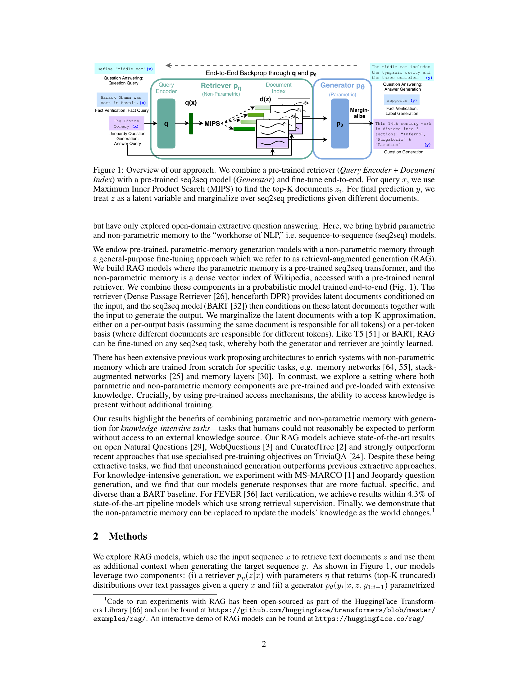
RAG combines both: a parametric generator (BART, a 400M-parameter seq2seq transformer) with a non-parametric retriever (a searchable index of 21 million Wikipedia passages). The generator provides language understanding and fluent output; the retriever provides access to up-to-date, verifiable facts.

The paper’s Figure 1 shows the full RAG architecture – a query encoder retrieves documents from an index, and the generator produces output conditioned on those documents:

Worked Example

Consider three questions and how parametric vs non-parametric memory handles them:

The key insight: RAG’s 626M trainable parameters outperformed T5’s 11B parameters on factual QA benchmarks (44.5 vs 34.5 Exact Match – a scoring metric where a prediction counts as correct only if it exactly matches the gold answer string – on Natural Questions). Giving a smaller model access to external knowledge beat making a larger model memorize everything – roughly 18 times fewer parameters for better results.

Exercises

Recall: What are the three problems with parametric memory that motivate RAG?

Apply: A company trains a customer-support chatbot in January. In March, they release a new product. Explain how a parametric-only model and a RAG model would each handle questions about the new product. Which requires retraining?

Extend: RAG uses Wikipedia as its knowledge source. What would happen if you replaced the Wikipedia index with a company’s internal documentation? What stays the same about the architecture, and what changes?

Lesson 2: Dense Passage Retrieval

RAG needs to find the most relevant documents from 21 million Wikipedia passages in milliseconds. This lesson explains how Dense Passage Retrieval (DPR) encodes both queries and documents as vectors and uses dot-product similarity to find matches.

Explanation

Imagine a library where every book has a GPS coordinate, and your question also has a GPS coordinate. To find relevant books, you calculate the distance from your question’s coordinate to every book’s coordinate and pick the closest ones. Dense passage retrieval works the same way, except the “coordinates” are high-dimensional vectors and “distance” is measured by dot product.

DPR uses a bi-encoder architecture (two separate encoders – one for queries and one for documents – that produce vectors in the same space). One BERT encoder (see BERT) converts the input query \(x\) into a vector \(\mathbf{q}(x)\), and a second BERT encoder converts each document \(z\) into a vector \(\mathbf{d}(z)\):

\[\mathbf{d}(z) = \text{BERT}_d(z), \quad \mathbf{q}(x) = \text{BERT}_q(x)\]

• \(\text{BERT}_d\) is the document encoder – a BERT-base model that reads a passage and outputs a single vector
• \(\text{BERT}_q\) is the query encoder – a separate BERT-base model that reads the input question and outputs a single vector
• Both vectors live in the same \(d\)-dimensional space (768 dimensions for BERT-base)

The retriever scores each document by the dot product between its vector and the query vector, then converts scores to probabilities:

\[p_\eta(z|x) \propto \exp\left(\mathbf{d}(z)^\top \mathbf{q}(x)\right)\]

• \(\mathbf{d}(z)^\top \mathbf{q}(x)\) is the dot product (inner product) between the document and query vectors
• \(\exp(\cdot)\) is the exponential function
• \(\propto\) means “proportional to” – the actual probability is computed by dividing by the sum of \(\exp(\mathbf{d}(z)^\top \mathbf{q}(x))\) over all documents (a softmax over the entire corpus)
• \(\eta\) represents the retriever parameters (the weights of both BERT encoders)

This is a softmax over dot-product scores: documents whose vectors point in a similar direction to the query vector get high probability. The model retrieves the top-\(K\) documents (typically \(K = 5\) or \(10\)) with the highest scores.

Why dot products? The critical efficiency advantage is that all 21 million document vectors \(\mathbf{d}(z)\) can be pre-computed once and stored in an index. At query time, only the query vector \(\mathbf{q}(x)\) needs to be computed, and finding the top-\(K\) documents becomes a Maximum Inner Product Search (MIPS) problem. The FAISS library (Facebook AI Similarity Search, a library for efficient similarity search over dense vectors) solves this with approximate nearest-neighbor algorithms in sub-linear time – meaning you do not need to scan all 21 million documents.

Worked Example

Suppose our query is “What is the capital of France?” and we have a tiny corpus of 3 documents, with embedding dimension \(d = 3\):

The query encoder produces \(\mathbf{q}(x) = [0.3, 0.8, 0.1]\).

Step 1: Compute dot products.

• \(\mathbf{d}(z_1)^\top \mathbf{q}(x) = 0.4 \times 0.3 + 0.7 \times 0.8 + 0.2 \times 0.1 = 0.12 + 0.56 + 0.02 = 0.70\)
• \(\mathbf{d}(z_2)^\top \mathbf{q}(x) = 0.3 \times 0.3 + 0.5 \times 0.8 + 0.6 \times 0.1 = 0.09 + 0.40 + 0.06 = 0.55\)
• \(\mathbf{d}(z_3)^\top \mathbf{q}(x) = 0.1 \times 0.3 + 0.2 \times 0.8 + 0.8 \times 0.1 = 0.03 + 0.16 + 0.08 = 0.27\)

Step 2: Exponentiate the scores.

• \(\exp(0.70) \approx 2.014\)
• \(\exp(0.55) \approx 1.733\)
• \(\exp(0.27) \approx 1.310\)

Step 3: Normalize to get probabilities.

\[\text{sum} = 2.014 + 1.733 + 1.310 = 5.057\]

• \(p_\eta(z_1|x) = 2.014 / 5.057 \approx 0.398\)
• \(p_\eta(z_2|x) = 1.733 / 5.057 \approx 0.343\)
• \(p_\eta(z_3|x) = 1.310 / 5.057 \approx 0.259\)

With \(K = 2\), the retriever selects \(z_1\) (Paris is the capital of France) and \(z_2\) (the Eiffel Tower in Paris) as the top-2 documents. Document \(z_3\) about Berlin scores lowest, as expected.

Exercises

Recall: Why does DPR use two separate BERT encoders instead of one shared encoder? What practical advantage does this provide?

Apply: Given query vector \(\mathbf{q} = [0.5, 0.3, 0.9]\) and two document vectors \(\mathbf{d}_1 = [0.4, 0.1, 0.8]\) and \(\mathbf{d}_2 = [0.9, 0.5, 0.1]\), compute the dot products and retriever probabilities. Which document is retrieved?

Extend: DPR pre-computes all document vectors offline. What happens if you want to add a new document to the index? What if you want to update the document encoder to produce better representations – how does that affect the index?

Lesson 3: Sequence-to-Sequence Generation

Once RAG retrieves relevant documents, it needs to generate an answer. This lesson explains how BART, a sequence-to-sequence transformer, reads an input (question + retrieved document) and produces text one token at a time.

Explanation

Think of a translator who reads an entire paragraph in French, forms an understanding of it, then writes the English translation word by word. As the translator writes each English word, they look back at their understanding of the French paragraph and at the English words they have already written. The BART generator works the same way: the encoder reads the input, the decoder produces the output one token at a time.

BART-large is a 400-million-parameter encoder-decoder transformer (see Attention Is All You Need). For RAG, the input to BART is the concatenation of the original query \(x\) and a retrieved document \(z\). The encoder processes this combined input and produces a sequence of hidden representations. The decoder then generates the output sequence \(y = (y_1, y_2, \ldots, y_N)\) token by token, where each token’s probability depends on:

\[p_\theta(y_i | x, z, y_{1:i-1})\]

• \(\theta\) represents the generator parameters (BART’s weights)
• \(x\) is the original input (the question)
• \(z\) is the retrieved document
• \(y_{1:i-1}\) are all previously generated tokens
• \(y_i\) is the current token being generated

This is autoregressive generation (producing a sequence one element at a time, where each element is conditioned on all previous elements). At each step, the decoder outputs a probability distribution over the entire vocabulary (around 50,000 tokens for BART). The model samples or selects the most likely token, appends it to the sequence, and continues until it generates a special end-of-sequence token.

Why concatenation? To combine the query and the retrieved document, RAG simply concatenates them as a single text string: “[query text] [document text]”. This concatenated string is fed to BART’s encoder. The self-attention mechanism in the encoder can then attend to both the question and the document, learning which parts of the document are relevant to the question. No architectural changes to BART are needed – it treats the concatenated input like any other text.

Worked Example

Suppose the query is “What is the capital of France?” and the retrieved document is “Paris is the capital and most populous city of France, with a population of 2.1 million.”

The encoder input is: “What is the capital of France? Paris is the capital and most populous city of France, with a population of 2.1 million.”

The decoder generates one token at a time. Suppose the vocabulary has tokens including “Paris”, “London”, “The”, “capital”, and many others. At the first step:

The model selects “Paris” (highest probability). Now at step 2, conditioned on \(y_1 = \text{"Paris"}\):

This continues until the model generates an end-of-sequence token, producing the complete answer “Paris”.

The key point: the generator assigns a probability to the complete output sequence by multiplying the per-token probabilities:

\[p_\theta(y | x, z) = \prod_{i=1}^{N} p_\theta(y_i | x, z, y_{1:i-1})\]

For our example: \(p_\theta(\text{"Paris"} | x, z) = 0.72 \times 0.15 = 0.108\) (if the end token has probability 0.15 after “Paris”). This sequence probability is what RAG uses when combining evidence from multiple documents.

Exercises

Recall: What does BART’s encoder receive as input in the RAG system, and why is simple concatenation sufficient?

Apply: Suppose the decoder produces the following per-token probabilities for the sequence “Paris is”: \(p(y_1 = \text{"Paris"}) = 0.72\), \(p(y_2 = \text{"is"} | y_1) = 0.45\), \(p(y_3 = \text{"\<end\>"} | y_1, y_2) = 0.20\). What is the probability of the complete sequence “Paris is”?

Extend: BART was pre-trained with a denoising objective – learning to reconstruct text that has been corrupted. How might this pre-training help with RAG’s task? Think about what skills denoising requires (understanding context, generating fluent text) and how they transfer.

Lesson 4: Marginalizing Over Latent Documents

This is the core innovation. RAG retrieves \(K\) documents, but which one should the generator use? Instead of picking the single best document, RAG treats the documents as latent variables (hidden choices that are not directly observed in the training data) and averages over all of them. This lesson explains the two marginalization strategies: RAG-Sequence and RAG-Token.

Explanation

Imagine you ask three friends the same question, and each friend has read a different reference book. Friend 1 says “Paris” with high confidence. Friend 2 says “Paris” with medium confidence. Friend 3 says “Lyon” with low confidence. To get your final answer, you could average their responses, weighting each by how relevant their reference book was. This is marginalization – summing out the “which friend” variable to get an overall answer probability.

In RAG, the “friends” are the \(K\) retrieved documents, and “how relevant their reference book was” is the retriever probability \(p_\eta(z|x)\). The model needs to combine the generation probabilities from all \(K\) documents into a single output distribution. RAG proposes two ways to do this.

RAG-Sequence: one document per answer. Each document generates the entire answer independently. The model then averages the complete-sequence probabilities weighted by the retriever scores:

\[p_{\text{RAG-Sequence}}(y|x) \approx \sum_{z \in \text{top-}k(p(\cdot|x))} p_\eta(z|x) \prod_{i}^{N} p_\theta(y_i|x, z, y_{1:i-1})\]

• The inner product \(\prod_{i}^{N} p_\theta(y_i|x, z, y_{1:i-1})\) computes the probability that the generator produces the entire sequence \(y\) when reading document \(z\)
• The outer sum \(\sum_{z}\) averages these sequence probabilities across documents, weighted by retriever scores \(p_\eta(z|x)\)
• This is like asking each friend to write a complete answer, then blending the answers by relevance

RAG-Token: one document per token. For each output token position, the model averages the per-token probabilities across all documents, then multiplies these averaged probabilities together:

\[p_{\text{RAG-Token}}(y|x) \approx \prod_{i}^{N} \sum_{z \in \text{top-}k(p(\cdot|x))} p_\eta(z|x) p_\theta(y_i|x, z, y_{1:i-1})\]

• The inner sum \(\sum_{z}\) computes a weighted average of the generation probabilities for token \(y_i\) across all documents
• The outer product \(\prod_{i}^{N}\) multiplies these per-token averages together
• This allows a single sentence to draw facts from multiple documents. Token 1 might be most influenced by document 3, while token 5 draws from document 1

The critical difference is the order of the product and sum. RAG-Sequence sums over documents outside the product (one document generates the whole answer). RAG-Token sums over documents inside the product (each token can use a different document).

Worked Example

Suppose \(K = 2\), and we want to compute the probability of the 2-token answer \(y = (y_1, y_2)\) = (“Paris”, “<end>”).

The retriever gives:

• \(p_\eta(z_1|x) = 0.6\) (document about France)
• \(p_\eta(z_2|x) = 0.4\) (document about European capitals)

The generator gives per-token probabilities:

RAG-Sequence – compute per-document sequence probabilities, then average:

• \(z_1\): \(p_\theta(y|x, z_1) = 0.80 \times 0.90 = 0.720\)
• \(z_2\): \(p_\theta(y|x, z_2) = 0.50 \times 0.70 = 0.350\)

\[p_{\text{RAG-Seq}}(y|x) = 0.6 \times 0.720 + 0.4 \times 0.350 = 0.432 + 0.140 = 0.572\]

RAG-Token – compute per-token weighted averages, then multiply:

• Token 1: \(\sum_z p_\eta(z|x) \cdot p_\theta(y_1|x, z) = 0.6 \times 0.80 + 0.4 \times 0.50 = 0.48 + 0.20 = 0.68\)
• Token 2: \(\sum_z p_\eta(z|x) \cdot p_\theta(y_2|x, z, y_1) = 0.6 \times 0.90 + 0.4 \times 0.70 = 0.54 + 0.28 = 0.82\)

\[p_{\text{RAG-Token}}(y|x) = 0.68 \times 0.82 = 0.558\]

The two approaches give different probabilities (0.572 vs 0.558) because they combine evidence differently. RAG-Sequence treats each document as a coherent hypothesis; RAG-Token allows mixing at the token level.

When does the difference matter? Consider generating a Jeopardy clue about Hemingway. RAG-Token might consult one document for “The Sun Also Rises” and a different document for “born in Oak Park, Illinois,” synthesizing information across documents within a single sentence. RAG-Sequence would need a single document that contains both facts.

Exercises

Recall: In the RAG-Sequence formula, what does the product \(\prod_{i}^{N}\) compute, and what does the sum \(\sum_{z}\) compute? Which operation is outermost?

Apply: Using the same retriever probabilities (\(p_\eta(z_1|x) = 0.6\), \(p_\eta(z_2|x) = 0.4\)), suppose the generator gives the following probabilities for the 3-token answer (“Paris”, “France”, “<end>”):

Compute \(p_{\text{RAG-Sequence}}(y|x)\) and \(p_{\text{RAG-Token}}(y|x)\).

Extend: If all \(K\) documents happen to produce exactly the same generation probabilities for every token, would RAG-Sequence and RAG-Token give the same result? Prove or disprove this mathematically.

Lesson 5: End-to-End Training

RAG has two components – retriever and generator – that need to work together. But nobody labels which document should be retrieved for each question. This lesson explains how RAG trains both components jointly using only question-answer pairs, with the retrieved documents treated as latent variables.

Explanation

Think of a research assistant and a writer working together on an article. The assistant finds reference materials, and the writer uses them to produce text. Nobody tells the assistant which references to find – the only feedback is whether the final article is good. If the article is good, the assistant learns that the references they found were useful. If the article is bad, the assistant adjusts their search strategy. Over time, the assistant learns what to look for based on what helps the writer produce better output.

In RAG, the retriever is the research assistant and the generator is the writer. The training objective is simple: minimize the negative log-likelihood of the correct answer \(y_j\) given the input \(x_j\), where the likelihood is computed using either the RAG-Sequence or RAG-Token formula:

\[\mathcal{L} = \sum_j -\log p(y_j|x_j)\]

• \((x_j, y_j)\) is the \(j\)-th input-output training pair (e.g., question and answer)
• \(p(y_j|x_j)\) is the marginalized probability from Lesson 4 – it already includes the sum over retrieved documents
• The sum is over all training examples
• This is minimized using Adam, a variant of stochastic gradient descent

The clever part is how gradients flow. When we compute \(-\log p(y_j|x_j)\) and differentiate, the gradients flow:

1. Through the generator (\(\theta\)): BART learns to better use the retrieved documents when generating answers. This is standard fine-tuning.
2. Through the query encoder (\(\eta\), specifically \(\text{BERT}_q\)): If a different query vector would retrieve documents that help the generator produce higher-probability answers, the gradient nudges the query encoder in that direction.

What does NOT get updated:

• The document encoder (\(\text{BERT}_d\)) is frozen. Updating it would require re-encoding all 21 million documents and rebuilding the FAISS index after each gradient step – prohibitively expensive.
• The document index is fixed during training (computed once from the frozen document encoder).

So RAG fine-tunes the query encoder and the entire BART generator, while keeping the document encoder and index fixed. The retriever improves by learning better queries, not by learning better document representations.

Worked Example

Suppose we have one training example: $x = $ “What is the capital of France?”, $y = $ “Paris”.

Step 1: The query encoder produces \(\mathbf{q}(x) = [0.3, 0.8, 0.1]\) and retrieves \(K = 2\) documents with probabilities \(p_\eta(z_1|x) = 0.6\) and \(p_\eta(z_2|x) = 0.4\).

Step 2: Using RAG-Token, suppose we compute \(p(y|x) = 0.558\) (from our Lesson 4 example).

Step 3: The loss is:

\[\mathcal{L} = -\log(0.558) \approx 0.584\]

Step 4: We compute gradients \(\frac{\partial \mathcal{L}}{\partial \theta}\) and \(\frac{\partial \mathcal{L}}{\partial \mathbf{q}(x)}\) and update parameters.

If the query encoder had produced a slightly different vector that gave more weight to \(z_1\) (the more relevant document), the generator would have assigned higher probability to “Paris,” the loss would have been lower, and the gradient signal reflects this. Over many training steps, the query encoder learns to retrieve documents that lead to correct answers.

Exercises

Recall: Which parameters are updated during RAG training and which are frozen? Why is the document encoder frozen?

Apply: Given two training examples with computed probabilities \(p(y_1|x_1) = 0.72\) and \(p(y_2|x_2) = 0.35\), compute the total loss \(\mathcal{L}\). Which example contributes more to the loss? What does that mean for gradient updates?

Extend: The authors kept the document encoder frozen and found this sufficient for strong performance. Under what circumstances might you expect updating the document encoder to be necessary? Think about the gap between the DPR pre-training domain (Wikipedia QA) and a potential target domain (e.g., medical literature).

Lesson 6: The Complete RAG System

This final lesson puts everything together: the full inference pipeline, decoding strategies, experimental results, and the critical ability to update knowledge by swapping the document index.

Explanation

The complete RAG pipeline for answering a question works as follows:

1. Encode the query: The query encoder (\(\text{BERT}_q\)) converts the input text into a vector \(\mathbf{q}(x)\).
2. Retrieve documents: FAISS searches the pre-computed document index to find the \(K\) documents with the highest dot-product scores against \(\mathbf{q}(x)\).
3. Generate with each document: For each of the \(K\) retrieved documents, BART encodes the concatenation of the query and the document, then the decoder produces output token probabilities.
4. Marginalize: The model combines the generation probabilities across all \(K\) documents using either RAG-Sequence or RAG-Token marginalization.
5. Decode: The final output text is produced from the marginalized probabilities.

Decoding differences. RAG-Token decoding is straightforward. Because the per-token marginalization produces a standard autoregressive transition probability:

\[p'_\theta(y_i|x, y_{1:i-1}) = \sum_{z \in \text{top-}k(p(\cdot|x))} p_\eta(z_i|x) p_\theta(y_i|x, z_i, y_{1:i-1})\]

This plugs directly into standard beam search (a decoding algorithm that keeps the top-\(B\) most likely partial sequences at each step) – no special decoding algorithm needed.

RAG-Sequence decoding is harder. The sequence-level marginalization does not decompose into per-token terms, so you cannot use a single beam search. Instead, the paper proposes two approaches:

• Thorough Decoding: Run beam search separately for each document, collect all candidate hypotheses, then re-score each hypothesis across all documents (running additional forward passes if needed) and sum the weighted probabilities.
• Fast Decoding: Same as Thorough Decoding but assume \(p_\theta(y|x, z) \approx 0\) for any hypothesis not generated in document \(z\)’s beam. This avoids extra forward passes at the cost of a looser approximation.

Results. RAG achieved state-of-the-art results on four open-domain QA benchmarks:

RAG-Sequence outperformed T5-11B on Natural Questions by 10 points with 18 times fewer trainable parameters. It also beat DPR, a specialized extractive QA system with a BERT cross-encoder re-ranker (a model that reads the query and document together in a single encoder to judge relevance, more accurate but slower than the bi-encoder retriever). Notably, RAG generated correct answers 11.8% of the time even when the gold answer did not appear verbatim in any retrieved document – something impossible for any extractive system.

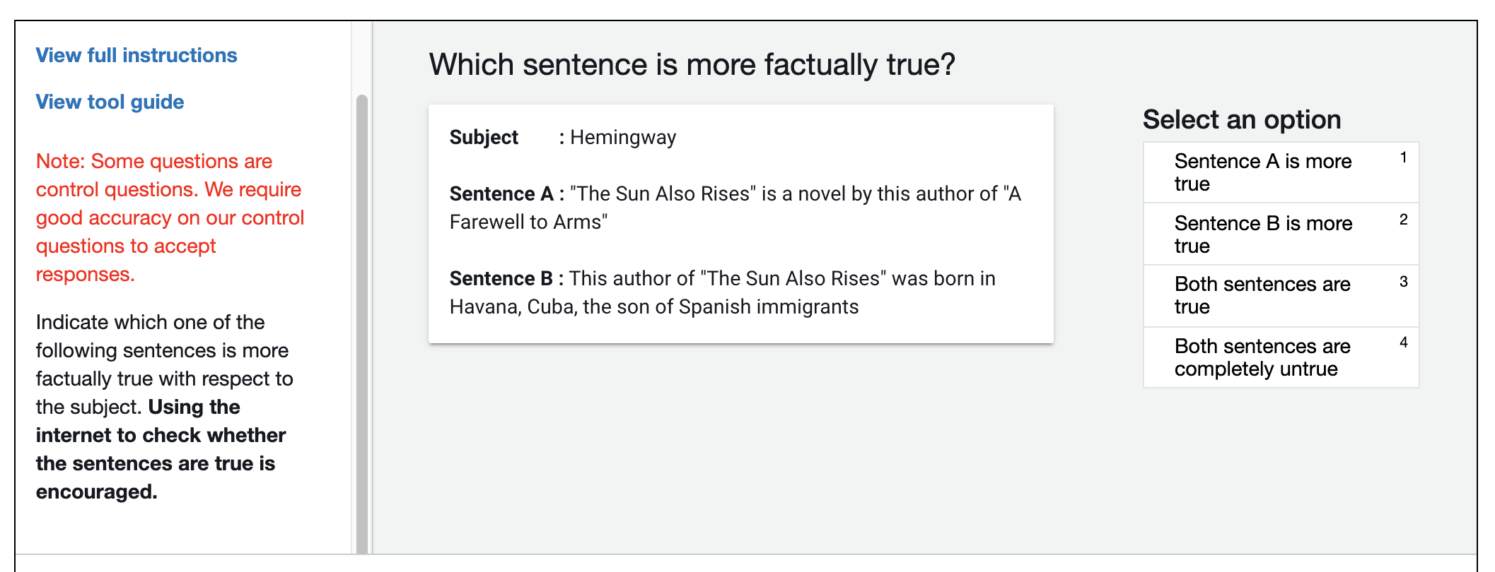
Figure 1: The annotation interface used for human evaluation of factuality. Evaluators compared pairs of generated sentences (one from BART, one from RAG) and judged which was more factually true, verifying claims using the internet. RAG was judged more factual in 42.7% of comparisons versus 7.1% for BART.

For text generation, RAG produced substantially more factual and diverse text than the BART baseline. On Jeopardy question generation, the ratio of distinct trigrams (three-word sequences) to total trigrams was 53.8% for RAG-Sequence versus 32.4% for BART, approaching the 90.0% diversity of human-written questions.

Index hot-swapping. One of the most consequential demonstrations in the paper is that RAG’s knowledge can be updated without retraining. The authors built two document indexes from Wikipedia snapshots taken at different dates and showed that swapping the index changed the model’s answers to reflect the newer information. This property – separating what the model knows from how the model reasons – became the foundation for how RAG is used in practice.

Limitations. RAG has important limitations:

• Single-hop retrieval: The model retrieves documents once and cannot issue follow-up queries. Multi-hop questions (“What is the capital of the country that won the 2018 World Cup?”) require chaining retrievals, which RAG does not support.
• Frozen document encoder: The document representations are fixed from DPR pre-training. Documents that DPR represents poorly (e.g., highly technical text, code, tables) may never be retrieved effectively.
• Retrieval collapse: On tasks without a clear need for factual knowledge (e.g., story generation), the retriever may learn to retrieve the same documents regardless of input, and the generator learns to ignore them.
• Wikipedia only: All experiments used English Wikipedia. Extending to other corpora, languages, or domains requires building new indexes.

Worked Example

Let us trace a complete RAG-Token inference with \(K = 2\) for the question “Who painted the Mona Lisa?”

Step 1 – Retrieve:

• \(z_1\): “The Mona Lisa is a half-length portrait painting by Italian artist Leonardo da Vinci.” (\(p_\eta = 0.65\))
• \(z_2\): “Leonardo da Vinci was an Italian polymath of the High Renaissance.” (\(p_\eta = 0.35\))

Step 2 – Generate per-token probabilities:

Step 3 – Marginalize per token:

• \(p'(y_1) = 0.65 \times 0.85 + 0.35 \times 0.70 = 0.553 + 0.245 = 0.798\)
• \(p'(y_2) = 0.65 \times 0.92 + 0.35 \times 0.88 = 0.598 + 0.308 = 0.906\)
• \(p'(y_3) = 0.65 \times 0.95 + 0.35 \times 0.91 = 0.618 + 0.319 = 0.936\)
• \(p'(y_4) = 0.65 \times 0.80 + 0.35 \times 0.75 = 0.520 + 0.263 = 0.783\)

Step 4 – Sequence probability:

\[p_{\text{RAG-Token}}(y|x) = 0.798 \times 0.906 \times 0.936 \times 0.783 \approx 0.530\]

The model produces “Leonardo da Vinci” with about 53% probability, drawing supporting evidence from both documents.

Exercises

Recall: What are the five steps in the RAG inference pipeline? Which step differs between RAG-Sequence and RAG-Token?

Apply: Using the worked example above, compute the RAG-Sequence probability for the same answer “Leonardo da Vinci” and compare it to the RAG-Token result.

Extend: The index hot-swapping experiment shows RAG can update its knowledge without retraining. But what about the query encoder – it was fine-tuned on the old index. Could there be a mismatch between the fine-tuned query encoder and a new document index? Under what conditions would this be a problem, and how might you mitigate it?

Comprehension Questions

1. RAG treats retrieved documents as latent variables. What does “latent” mean in this context, and why is this approach better than requiring explicit labels for which document to retrieve?

2. Why did the authors choose to freeze the document encoder during training instead of updating it? What is the computational cost of updating it, and when might it be worth paying that cost?

3. Compare RAG to DPR (a purely extractive system). RAG generated correct answers 11.8% of the time even when the answer did not appear in any retrieved document. How is this possible, and why can extractive systems never do this?

4. The authors observed “retrieval collapse” on story generation tasks, where the retriever learned to always retrieve the same documents. Why does this happen, and what does it tell us about the types of tasks where RAG works well vs poorly?

5. RAG builds on both BERT (see BERT) and the Transformer encoder-decoder architecture (see Attention Is All You Need). If you replaced BART with a decoder-only model like GPT (see Improving Language Understanding by Generative Pre-Training), what architectural changes would be needed and what capabilities might change?

Hands-On Project

Goal

Build a minimal RAG system from scratch using numpy. You will implement the bi-encoder retriever, the autoregressive generator (with pre-set weights), and both marginalization strategies (RAG-Sequence and RAG-Token).

Specification

• Implement document and query encoding as simple matrix multiplications (simulating BERT encoders)
• Build a retriever that computes dot-product scores and returns top-K documents
• Implement an autoregressive generator that produces per-token probabilities conditioned on a document
• Compute output probabilities using both RAG-Sequence and RAG-Token marginalization
• Demonstrate that RAG-Token allows different tokens to draw from different documents
• Use toy data: 5 documents, vocabulary of 10 tokens, embedding dimension 4

Starter Code

import numpy as np

np.random.seed(42)

# --- Configuration ---
VOCAB_SIZE = 10
EMBED_DIM = 4
NUM_DOCS = 5
K = 3  # top-K documents to retrieve
MAX_SEQ_LEN = 4  # maximum output length

# Token vocabulary
VOCAB = ["paris", "france", "capital", "berlin", "germany",
         "london", "england", "city", "is", "<end>"]

# --- Document corpus ---
# Each document is represented as a pre-computed embedding vector (simulating BERT_d output)
# In a real system, these would be produced by a BERT encoder
doc_texts = [
    "Paris is the capital of France",
    "Berlin is the capital of Germany",
    "London is the capital of England",
    "France is a country in Europe",
    "The Eiffel Tower is in Paris",
]
doc_embeddings = np.array([
    [0.9, 0.3, 0.1, 0.2],   # doc 0: Paris/France/capital
    [0.1, 0.8, 0.2, 0.3],   # doc 1: Berlin/Germany/capital
    [0.2, 0.1, 0.9, 0.1],   # doc 2: London/England/capital
    [0.7, 0.2, 0.0, 0.5],   # doc 3: France general
    [0.8, 0.1, 0.1, 0.4],   # doc 4: Eiffel Tower/Paris
])

# --- Query encoder weights (simulating BERT_q) ---
# Maps a one-hot query ID to an embedding vector
query_weight = np.array([
    [0.8, 0.2, 0.1, 0.3],   # query 0: "What is the capital of France?"
])


def retrieve_top_k(query_embedding, doc_embeddings, k):
    """
    Compute dot-product scores between query and all documents.
    Return indices of top-k documents and their probabilities.

    Args:
        query_embedding: shape (EMBED_DIM,)
        doc_embeddings: shape (NUM_DOCS, EMBED_DIM)
        k: number of documents to retrieve

    Returns:
        top_k_indices: shape (k,) -- indices of top-k documents
        top_k_probs: shape (k,) -- retriever probabilities (softmax over top-k scores)
    """
    # TODO: Compute dot products between query and each document
    # TODO: Find top-k indices
    # TODO: Apply softmax to top-k scores to get probabilities
    # Hint: softmax(z_i) = exp(z_i) / sum(exp(z_j)) over the top-k scores only
    pass


def generator_probs(doc_index, token_index, prev_tokens):
    """
    Simulate the generator (BART) producing per-token probabilities.
    In a real system, this would be a full transformer forward pass.
    Here we use a hand-crafted probability table.

    Args:
        doc_index: which retrieved document is being conditioned on
        token_index: which token position (0-indexed)
        prev_tokens: list of previously generated token indices

    Returns:
        probs: shape (VOCAB_SIZE,) -- probability distribution over vocabulary
    """
    # Pre-defined generation probabilities for "What is the capital of France?"
    # conditioned on different documents
    #
    # VOCAB: ["paris", "france", "capital", "berlin", "germany",
    #         "london", "england", "city", "is", "<end>"]

    # Document 0: "Paris is the capital of France" -> strongly generates "paris"
    # Document 3: "France is a country in Europe" -> weakly generates "paris"
    # Document 4: "Eiffel Tower is in Paris" -> medium generates "paris"
    gen_table = {
        # doc_index: {token_position: probability distribution over vocab}
        0: {  # Paris/France/capital doc
            0: [0.75, 0.05, 0.05, 0.02, 0.01, 0.02, 0.01, 0.02, 0.02, 0.05],
            1: [0.02, 0.02, 0.02, 0.01, 0.01, 0.01, 0.01, 0.02, 0.03, 0.85],
        },
        3: {  # France general doc
            0: [0.45, 0.15, 0.10, 0.05, 0.03, 0.05, 0.02, 0.05, 0.03, 0.07],
            1: [0.03, 0.03, 0.03, 0.02, 0.02, 0.02, 0.02, 0.03, 0.05, 0.75],
        },
        4: {  # Eiffel Tower/Paris doc
            0: [0.60, 0.05, 0.05, 0.03, 0.02, 0.03, 0.02, 0.05, 0.05, 0.10],
            1: [0.03, 0.02, 0.02, 0.01, 0.01, 0.02, 0.01, 0.03, 0.05, 0.80],
        },
    }

    probs = gen_table.get(doc_index, {}).get(token_index)
    if probs is None:
        # Default: uniform distribution (unknown doc/position)
        return np.ones(VOCAB_SIZE) / VOCAB_SIZE
    return np.array(probs)


def rag_sequence(query_embedding, doc_embeddings, target_tokens, k):
    """
    Compute RAG-Sequence probability: marginalize over documents at the sequence level.

    p_RAG-Seq(y|x) = sum_z p(z|x) * prod_i p(y_i|x,z,y_{<i})

    Args:
        query_embedding: shape (EMBED_DIM,)
        doc_embeddings: shape (NUM_DOCS, EMBED_DIM)
        target_tokens: list of token indices for the target sequence (e.g., [0, 9] for "paris <end>")
        k: number of documents to retrieve

    Returns:
        prob: the RAG-Sequence probability of the target sequence
    """
    top_k_indices, top_k_probs = retrieve_top_k(query_embedding, doc_embeddings, k)

    # TODO: For each retrieved document, compute the full sequence probability
    # TODO: Weight by retriever probability and sum
    pass


def rag_token(query_embedding, doc_embeddings, target_tokens, k):
    """
    Compute RAG-Token probability: marginalize over documents at the token level.

    p_RAG-Token(y|x) = prod_i sum_z p(z|x) * p(y_i|x,z,y_{<i})

    Args:
        query_embedding: shape (EMBED_DIM,)
        doc_embeddings: shape (NUM_DOCS, EMBED_DIM)
        target_tokens: list of token indices for the target sequence (e.g., [0, 9] for "paris <end>")
        k: number of documents to retrieve

    Returns:
        prob: the RAG-Token probability of the target sequence
    """
    top_k_indices, top_k_probs = retrieve_top_k(query_embedding, doc_embeddings, k)

    # TODO: For each token position, compute the weighted average probability across documents
    # TODO: Multiply the per-token marginals together
    pass


# --- Main ---
if __name__ == "__main__":
    query_emb = query_weight[0]  # embedding for "What is the capital of France?"

    # Step 1: Retrieve top-K documents
    top_k_idx, top_k_p = retrieve_top_k(query_emb, doc_embeddings, K)
    print("=== Retrieval ===")
    for rank, (idx, prob) in enumerate(zip(top_k_idx, top_k_p)):
        print(f"  Rank {rank+1}: doc {idx} (p={prob:.4f}) \"{doc_texts[idx]}\"")

    # Step 2: Compute RAG probabilities for target "paris <end>" (token indices [0, 9])
    target = [0, 9]  # "paris", "<end>"
    target_str = " ".join(VOCAB[t] for t in target)

    p_seq = rag_sequence(query_emb, doc_embeddings, target, K)
    p_tok = rag_token(query_emb, doc_embeddings, target, K)

    print(f"\n=== Target: \"{target_str}\" ===")
    print(f"  RAG-Sequence probability: {p_seq:.6f}")
    print(f"  RAG-Token probability:    {p_tok:.6f}")

    # Step 3: Compare per-token contributions to show RAG-Token's document mixing
    print("\n=== Per-Token Analysis (RAG-Token) ===")
    for i, t in enumerate(target):
        print(f"  Token {i} (\"{VOCAB[t]}\"):")
        for rank, (idx, prob) in enumerate(zip(top_k_idx, top_k_p)):
            gen_p = generator_probs(idx, i, target[:i])
            print(f"    doc {idx}: retriever_p={prob:.4f} * generator_p={gen_p[t]:.4f} = {prob * gen_p[t]:.4f}")

    # Step 4: Show that the loss would be
    loss = -np.log(p_seq)
    print(f"\n=== Training Loss (RAG-Sequence) ===")
    print(f"  -log p(y|x) = {loss:.6f}")

Expected Output

=== Retrieval ===
  Rank 1: doc 0 (p=0.4191) "Paris is the capital of France"
  Rank 2: doc 4 (p=0.3379) "The Eiffel Tower is in Paris"
  Rank 3: doc 3 (p=0.2430) "France is a country in Europe"

=== Target: "paris <end>" ===
  RAG-Sequence probability: 0.521498
  RAG-Token probability:    0.523498

=== Per-Token Analysis (RAG-Token) ===
  Token 0 ("paris"):
    doc 0: retriever_p=0.4191 * generator_p=0.7500 = 0.3143
    doc 4: retriever_p=0.3379 * generator_p=0.6000 = 0.2027
    doc 3: retriever_p=0.2430 * generator_p=0.4500 = 0.1094
  Token 1 ("<end>"):
    doc 0: retriever_p=0.4191 * generator_p=0.8500 = 0.3562
    doc 4: retriever_p=0.3379 * generator_p=0.8000 = 0.2703
    doc 3: retriever_p=0.2430 * generator_p=0.7500 = 0.1823

=== Training Loss (RAG-Sequence) ===
  -log p(y|x) = 0.651522

Further Reading

• DPR (Karpukhin et al., 2020) – the dense passage retrieval system that RAG’s retriever is based on. Explains how the bi-encoder is trained and how MIPS is used for efficient search.
• BART (Lewis et al., 2019) – the sequence-to-sequence model used as RAG’s generator. Covers the denoising pre-training objective and generation capabilities.
• REALM (Guu et al., 2020) – an earlier retrieval-augmented model that does update the document encoder during pre-training, using an asynchronous index refresh. Compare with RAG’s decision to keep the document encoder frozen.
• Fusion-in-Decoder (Izacard & Grave, 2021) – an alternative approach where all retrieved documents are concatenated and fed to the encoder simultaneously, rather than processed independently. Achieved stronger QA results than RAG.
• RETRO (Borgeaud et al., 2022) – scales retrieval-augmented generation to much larger models and corpora, retrieving chunks during both pre-training and inference.
• Self-RAG (Asai et al., 2023) – teaches the model to decide when retrieval is needed and to critique its own retrieved evidence, addressing RAG’s limitation of always retrieving the same number of documents.