Self-Consistency Improves Chain of Thought Reasoning in Language Models: Course

Learning Objectives

By the end of this course, you will be able to:

1. Explain how autoregressive language models generate text and why different decoding strategies (greedy, temperature sampling, top-k) produce different outputs from the same model
2. Describe how chain-of-thought prompting decomposes reasoning into intermediate steps and why greedy decoding limits it to a single reasoning path
3. Implement majority voting over a set of candidate answers and explain why it filters out errors
4. Compute length-normalized conditional probabilities for generated sequences and explain why normalization matters
5. Apply the full self-consistency pipeline – sample diverse reasoning paths, parse final answers, aggregate by majority vote – and explain why correct reasoning paths converge while incorrect ones scatter

Prerequisites

• Autoregressive language models – how models generate text one token at a time, with each token conditioned on all previous tokens. Covered in the GPT course (see Improving Language Understanding by Generative Pre-Training).
• The transformer architecture – the neural network architecture underlying all models in this paper. Covered in the Transformers course (see Attention Is All You Need).
• Chain-of-thought prompting – augmenting few-shot exemplars with step-by-step reasoning to improve multi-step problem solving. Covered in the CoT course (see Chain-of-Thought Prompting Elicits Reasoning in Large Language Models).
• Basic probability – conditional probability, products of probabilities, geometric means, the indicator function.

Lesson 1: Decoding Strategies – How a Model Chooses Its Words

Before you can understand self-consistency, you need to understand the mechanism it exploits: the fact that a language model does not have to give the same answer every time. The way you extract text from a model – the decoding strategy – determines whether the output is fixed or variable.

Explanation

Think about ordering coffee at a cafe. If you always order “the usual,” you get the same drink every time – that is greedy decoding. But if you tell the barista “surprise me with something I’d probably like,” you get a different drink each visit, weighted toward your known preferences – that is sampling. Both approaches use the same menu (the model’s probability distribution), but they produce different outputs.

An autoregressive language model generates text one token at a time. At each step, the model outputs a probability distribution over its entire vocabulary – every possible next word gets a probability. The decoding strategy decides how to pick the actual next token from this distribution.

Greedy decoding always picks the single most probable token at each step:

\[t_k = \arg\max_{t} P(t \mid t_1, t_2, \ldots, t_{k-1})\]

where:

• \(t_k\) is the token selected at step \(k\)
• \(P(t \mid t_1, \ldots, t_{k-1})\) is the probability the model assigns to token \(t\) given all previously generated tokens
• \(\arg\max\) selects the token with the highest probability

Greedy decoding is deterministic: given the same input, the model always produces the same output. This means you get exactly one reasoning path per question.

Temperature sampling introduces controlled randomness. Before sampling, the model divides each log-probability by a temperature parameter \(T\):

\[P_T(t \mid t_1, \ldots, t_{k-1}) = \frac{\exp(\log P(t \mid t_1, \ldots, t_{k-1}) / T)}{\sum_{t'} \exp(\log P(t' \mid t_1, \ldots, t_{k-1}) / T)}\]

where:

• \(T\) is the temperature parameter (a positive number)
• When \(T = 1\), this reduces to the original distribution
• When \(T < 1\), the distribution becomes “sharper” – high-probability tokens get even higher probability, making sampling more deterministic
• When \(T > 1\), the distribution becomes “flatter” – low-probability tokens get relatively more likely, increasing diversity

The self-consistency paper uses temperatures between 0.3 and 0.7, which produce moderate diversity: enough variation to explore different reasoning paths, but not so much that the model generates nonsense.

Top-k sampling restricts the candidate set to the \(k\) most probable tokens, then samples from those:

\[P_{\text{top-k}}(t) = \begin{cases} \frac{P(t)}{\sum_{t' \in \text{top-k}} P(t')} & \text{if } t \in \text{top-k tokens} \\ 0 & \text{otherwise} \end{cases}\]

where:

• \(k\) is a fixed number (the paper uses \(k = 40\))
• Only the \(k\) highest-probability tokens are eligible for selection
• Their probabilities are renormalized so they sum to 1

Top-k prevents the model from selecting very unlikely tokens (which could derail the reasoning) while still allowing diversity among the plausible options.

Worked Example

Suppose a model is generating text and, at the current step, the probability distribution over a small vocabulary of 5 tokens is:

Greedy decoding always picks “eggs” (probability 0.45).

Temperature sampling with \(T = 0.5\): We compute new probabilities by dividing log-probs by \(T = 0.5\) (equivalently, squaring then renormalizing):

• “eggs”: \(0.45^{1/0.5} = 0.45^2 = 0.2025\)
• “ducks”: \(0.25^2 = 0.0625\)
• “hens”: \(0.15^2 = 0.0225\)
• “birds”: \(0.10^2 = 0.0100\)
• “geese”: \(0.05^2 = 0.0025\)

Sum = 0.3000. After renormalizing:

The distribution is sharper: “eggs” jumped from 45% to 67.5%, while “geese” dropped from 5% to 0.8%. Sampling from this distribution usually picks “eggs” but sometimes picks “ducks” or “hens” – introducing variety without chaos.

Top-k with \(k = 3\): Only “eggs,” “ducks,” and “hens” are eligible. Renormalized:

“birds” and “geese” are excluded entirely.

Exercises

Recall: What is the key difference between greedy decoding and temperature sampling? Which one produces the same output every time?

Apply: Given the vocabulary probabilities [0.50, 0.30, 0.15, 0.05], compute the temperature-adjusted probabilities for \(T = 2.0\). (Hint: raise each probability to the power \(1/T = 0.5\), i.e., take square roots, then renormalize.) How does this distribution compare to the original?

Extend: If you set the temperature \(T\) extremely high (say \(T = 100\)), what does the distribution approach? If you set \(T\) extremely close to 0, what does the distribution approach? Relate these extremes to uniform random sampling and greedy decoding.

Lesson 2: The Problem with a Single Reasoning Path

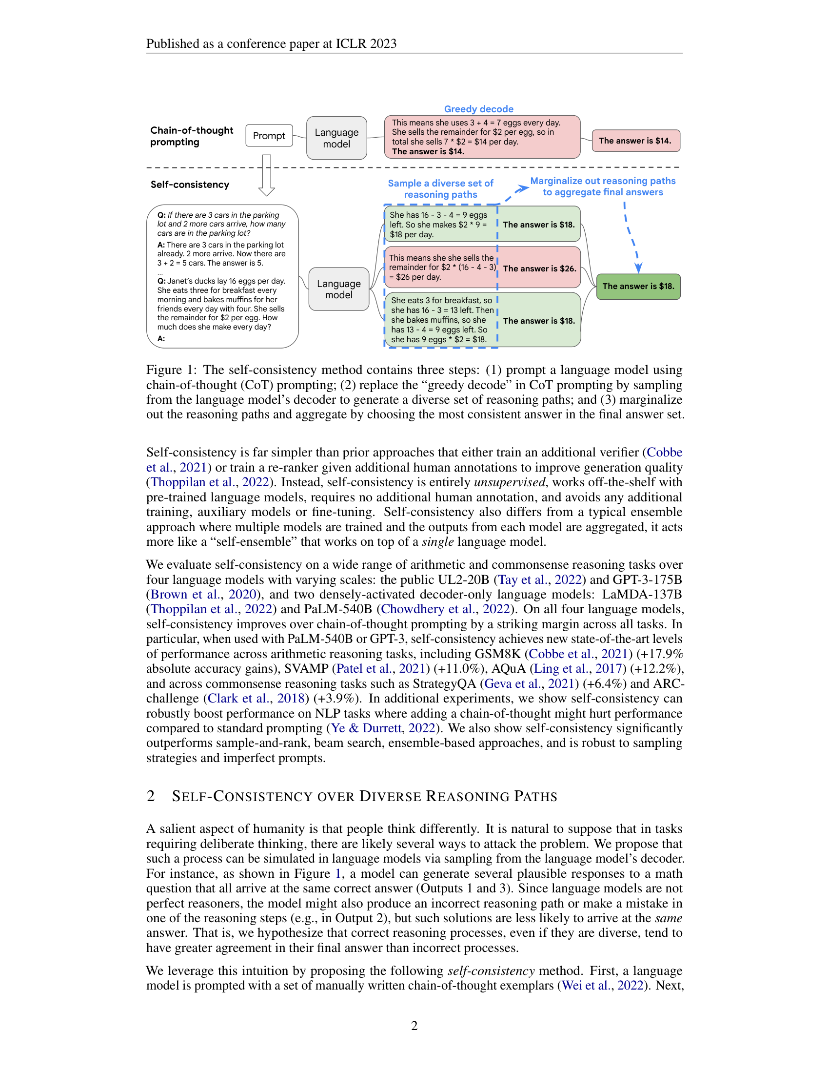
Chain-of-thought prompting (see Chain-of-Thought Prompting Elicits Reasoning in Large Language Models) was a breakthrough: by showing a language model step-by-step reasoning in the prompt exemplars, the model learns to “show its work” before answering. But standard CoT uses greedy decoding, which means it commits to exactly one chain of reasoning. This lesson examines why that is a fundamental limitation.

Explanation

Imagine you are taking a math exam and you are only allowed to write one solution attempt per problem. If you make a small mistake in step 2 of a 5-step problem – say, you subtract instead of add – every subsequent step builds on that error. You cannot recover. Your final answer is wrong, and you have no second chance.

This is exactly what happens with chain-of-thought prompting under greedy decoding. The model produces one reasoning chain, token by token, left to right. If it makes an error at any step – misreading the problem, choosing the wrong operation, making an arithmetic mistake – every subsequent token is conditioned on that error. The model has locked itself into a single path and cannot backtrack.

Consider this example from the paper. The question: “Janet’s ducks lay 16 eggs per day. She eats 3 for breakfast and bakes muffins with 4. She sells the rest for $2 each. How much does she make daily?”

The greedy decoding path from LaMDA-137B produces:

“She eats 3 + 4 = 7 eggs every day. She sells the remainder for $2 per egg, so in total she sells 7 * $2 = $14 per day. The answer is $14.”

The error occurs in the last computation: the model computes the number of eggs used (7) but then multiplies that by $2, instead of computing the remainder (16 - 7 = 9) and multiplying by $2. The model correctly identified that 3 + 4 = 7 eggs are used, but then confused “eggs used” with “eggs sold.” Once this confusion enters the reasoning chain, greedy decoding has no mechanism to revisit it.

The paper found this problem is pervasive. On the GSM8K benchmark (grade-school math word problems), CoT prompting with greedy decoding achieves 56.5% accuracy on PaLM-540B. That means the model gets 43.5% of problems wrong – often due to a single misstep in an otherwise correct reasoning chain.

The fundamental issue is not that the model lacks the ability to reason correctly. If you ask the same model the same question multiple times using sampling instead of greedy decoding, it often produces the correct reasoning in some of those attempts. The knowledge is there; greedy decoding just does not explore enough of the space to reliably surface it.

Worked Example

Let’s trace three hypothetical reasoning paths for the duck-eggs problem to see how diversity helps.

Question: “Janet’s ducks lay 16 eggs per day. She eats 3 for breakfast and bakes muffins with 4. She sells the rest for $2 each. How much does she make daily?”

Correct answer: 16 - 3 - 4 = 9 eggs sold, 9 * $2 = $18.

Path 1 (greedy decode):

• “She eats 3 + 4 = 7 eggs.”
• “She sells 7 * $2 = $14.”
• Answer: $14 (wrong – confused “used” with “sold”)

Path 2 (sampled):

• “She has 16 - 3 - 4 = 9 eggs left.”
• “She makes 9 * $2 = $18.”
• Answer: $18 (correct)

Path 3 (sampled):

• “She eats 3, leaving 16 - 3 = 13.”
• “She bakes with 4, leaving 13 - 4 = 9.”
• “She sells 9 eggs at $2 each: 9 * $2 = $18.”
• Answer: $18 (correct – different reasoning route, same answer)

Paths 2 and 3 take different routes (one subtracts both at once, the other subtracts sequentially) but arrive at the same answer. Path 1 makes a different kind of error. If we only had Path 1 (greedy decoding), we would get the wrong answer. If we have all three paths, two out of three say $18 – the correct answer wins.

Exercises

Recall: Why can’t greedy decoding recover from an error made early in the reasoning chain?

Apply: For the following problem, write two different valid reasoning paths that arrive at the same correct answer: “A store has 5 boxes. Each box contains 8 apples. A customer buys 12 apples. How many apples remain?”

Extend: The paper reports that self-consistency helps even when CoT prompting hurts performance compared to standard prompting (e.g., on ANLI-R1: standard prompting 69.1%, CoT 68.8%, self-consistency 78.5%). How can sampling multiple CoT paths and voting outperform standard prompting if a single CoT path does worse?

Lesson 3: Majority Voting – The Wisdom of Crowds

The core mechanism of self-consistency is majority voting: sample many answers and pick the one that appears most often. This lesson formalizes how majority voting works and why it reliably filters out errors when the correct answer is more consistent than any individual wrong answer.

Explanation

Suppose you are lost in a city and ask 10 strangers for directions to the train station. Seven say “go north,” two say “go east,” and one says “go south.” You would head north, not because any single person is guaranteed to be right, but because the correct answer attracts more agreement than any particular wrong answer.

This is exactly the principle behind self-consistency. Each sampled reasoning path is like asking a different “stranger” – the stochastic (randomly determined) sampling process means each path might take a different approach, make different mistakes, or arrive at a different answer. The key insight is that correct reasoning paths, despite taking different routes, tend to converge on the same answer. Wrong reasoning paths, by contrast, tend to scatter across multiple different wrong answers.

The majority vote formula is:

\[a^* = \arg\max_a \sum_{i=1}^{m} \mathbb{1}(a_i = a)\]

where:

• \(a^*\) is the final selected answer
• \(a\) ranges over all distinct answers that appear in the \(m\) samples
• \(m\) is the total number of sampled reasoning paths (the paper typically uses \(m = 40\))
• \(a_i\) is the final answer parsed from the \(i\)-th sampled reasoning path
• \(\mathbb{1}(a_i = a)\) is the indicator function: equals 1 if \(a_i = a\), and 0 otherwise

In plain language: count how many times each answer appears across all sampled paths, then pick the answer with the highest count.

Why does this work? It rests on a statistical assumption: the probability that the model produces the correct answer on any given sample is higher than the probability of any specific wrong answer. If the model has a 40% chance of producing the correct answer and a 60% chance of being wrong, but those wrong answers are spread across 10 different incorrect values (each around 6%), then the correct answer will dominate the vote even though the model is wrong more often than right on any single attempt.

The paper demonstrates that this assumption holds in practice. On GSM8K with PaLM-540B, greedy decoding gets 56.5% accuracy (each individual sample is correct a bit more than half the time), but self-consistency with 40 samples reaches 74.4%. The 18-point gap comes from situations where the model was wrong on its greedy path but correct on enough sampled paths for the majority vote to recover.

Worked Example

Suppose we sample \(m = 7\) reasoning paths for a math problem where the correct answer is 42. The sampled answers are:

Now apply the majority vote formula. Count each answer:

• \(\sum_{i=1}^{7} \mathbb{1}(a_i = 42) = 4\) (paths 1, 3, 4, 7)
• \(\sum_{i=1}^{7} \mathbb{1}(a_i = 38) = 2\) (paths 2, 6)
• \(\sum_{i=1}^{7} \mathbb{1}(a_i = 50) = 1\) (path 5)

\[a^* = \arg\max_a \{4, 2, 1\} = 42\]

The majority vote correctly selects 42 with 4 out of 7 votes. Notice that the model was wrong 3 out of 7 times (43% error rate on individual samples), but the wrong answers split between 38 and 50, so neither wrong answer accumulated enough votes to overtake the correct one.

Now consider a harder case: same problem, but the model is less reliable.

Counts: 42 gets 3, 38 gets 3, 50 gets 1. This is a tie between 42 and 38. In a tie, the paper takes the answer encountered first. But the real lesson here is that with only 7 samples, ties can happen. Increasing \(m\) reduces the chance of ties and makes the vote more reliable. The paper uses \(m = 40\) in most experiments precisely to give the vote enough “resolution” to clearly separate the correct answer.

Exercises

Recall: What does the indicator function \(\mathbb{1}(a_i = a)\) compute? In the context of self-consistency, what role does it play?

Apply: You sample 10 reasoning paths and get answers: [18, 14, 18, 26, 18, 14, 18, 22, 14, 18]. Compute the majority vote. What fraction of samples produced the winning answer?

Extend: Majority voting fails when a specific wrong answer is more common than the correct answer. Give an example of a question type where this might happen (hint: think about common misconceptions or problems where a plausible-but-wrong reasoning step is more natural than the correct one).

Lesson 4: Sequence Probabilities and Weighted Voting

Majority voting treats all reasoning paths equally – each one gets exactly one vote regardless of how “confident” the model was in generating it. An alternative is to weight each path by its probability: paths the model considers more likely get more influence. This lesson explores weighted voting and explains why, surprisingly, it barely outperforms simple majority vote.

Explanation

Think about a jury deliberation. In a standard jury, each juror gets one vote regardless of expertise. But what if you could weight votes by each juror’s confidence level? A juror who says “I’m 95% sure” would count more than one who says “I’m 55% sure.” In theory, weighted voting should be more informative.

To implement weighted voting for self-consistency, you need to compute the probability that the model assigns to each generated reasoning path. An autoregressive model generates a sequence of tokens \(t_1, t_2, \ldots, t_K\) one at a time, and the total probability of the sequence is the product of each token’s conditional probability:

\[P(t_1, t_2, \ldots, t_K) = \prod_{k=1}^{K} P(t_k \mid t_1, \ldots, t_{k-1})\]

where:

• \(K\) is the total number of tokens in the output (reasoning path plus final answer)
• \(P(t_k \mid t_1, \ldots, t_{k-1})\) is the probability of the \(k\)-th token given all previous tokens

There is a problem: longer sequences have lower total probability because you are multiplying many numbers less than 1. A 50-token reasoning path will almost always have a lower probability than a 10-token path, even if the 50-token path is better reasoning. This unfairly penalizes detailed explanations.

The fix is length normalization. The paper uses the geometric mean of per-token probabilities:

\[P(\mathbf{r}_i, \mathbf{a}_i \mid \text{prompt}, \text{question}) = \exp\left(\frac{1}{K}\sum_{k=1}^{K} \log P(t_k \mid \text{prompt}, \text{question}, t_1, \ldots, t_{k-1})\right)\]

where:

• \(\mathbf{r}_i\) is the reasoning path in the \(i\)-th sample
• \(\mathbf{a}_i\) is the final answer in the \(i\)-th sample
• \(K\) is the total number of tokens in \((\mathbf{r}_i, \mathbf{a}_i)\)
• \(t_k\) is the \(k\)-th token in the sequence
• The \(\frac{1}{K}\) factor averages the log-probabilities, giving the geometric mean

This formula computes the average per-token log-probability, then exponentiates it. A longer sequence with high average per-token confidence scores just as well as a shorter one.

The weighted vote then becomes:

\[a^* = \arg\max_a \sum_{i=1}^{m} P(\mathbf{r}_i, \mathbf{a}_i \mid \text{prompt}, \text{question}) \cdot \mathbb{1}(a_i = a)\]

Instead of counting each vote as 1, each vote is weighted by its normalized probability.

Here is the surprising finding: in practice, weighted voting barely outperforms unweighted majority vote. On PaLM-540B across six benchmarks, unweighted majority vote and the normalized weighted sum achieve nearly identical accuracy (e.g., 74.4% vs. 74.1% on GSM8K, 99.3% vs. 99.3% on MultiArith). The reason is that the model assigns similar probabilities to all its generated paths – both correct and incorrect ones. The weights are approximately equal, so weighting has no effect.

This is an important insight about model calibration (how well a model’s confidence scores reflect its actual accuracy): language models are not good at distinguishing their own correct reasoning from incorrect reasoning based on probability alone. The model is just as “confident” in a wrong chain of thought as in a right one. This is precisely why external re-rankers and verifiers were trained in prior work – and why the simpler majority vote works just as well as the weighted version.

Worked Example

Suppose we sample 3 reasoning paths for a question. Each path has a different number of tokens and different per-token log-probabilities:

Path 1: 20 tokens, per-token log-probabilities sum to -8.0, answer = 18

• Average log-prob: \(-8.0 / 20 = -0.40\)
• Normalized probability: \(\exp(-0.40) = 0.670\)

Path 2: 35 tokens, per-token log-probabilities sum to -15.75, answer = 14

• Average log-prob: \(-15.75 / 35 = -0.45\)
• Normalized probability: \(\exp(-0.45) = 0.638\)

Path 3: 25 tokens, per-token log-probabilities sum to -10.0, answer = 18

• Average log-prob: \(-10.0 / 25 = -0.40\)
• Normalized probability: \(\exp(-0.40) = 0.670\)

Unweighted majority vote: Answer 18 gets 2 votes, answer 14 gets 1 vote. Winner: 18.

Weighted vote: Score for 18 = \(0.670 + 0.670 = 1.340\). Score for 14 = \(0.638\). Winner: 18.

Notice how the weights (0.670, 0.638, 0.670) are all close to each other. Path 2 is wrong but its probability is nearly the same as the correct paths. The weighted vote reaches the same conclusion as the unweighted vote because the model cannot reliably assign lower probability to incorrect reasoning.

Now compare what happens without length normalization. The unnormalized probabilities would be:

• Path 1: \(\exp(-8.0) = 0.000335\)
• Path 2: \(\exp(-15.75) = 0.00000014\)
• Path 3: \(\exp(-10.0) = 0.0000454\)

Path 2, with 35 tokens, has a vastly lower raw probability simply because it is longer. Unnormalized weighting dramatically distorts the vote. This is why the paper shows that unnormalized weighting performs much worse (e.g., 59.9% vs. 74.4% on GSM8K).

Exercises

Recall: Why does length normalization matter when computing sequence probabilities? What happens without it?

Apply: A reasoning path has 4 tokens with per-token log-probabilities [-0.3, -0.5, -0.2, -0.6]. Compute the length-normalized probability. Then compute the unnormalized probability (the product of all token probabilities). How different are they?

Extend: The paper finds that weighted voting performs almost identically to unweighted majority vote. Under what circumstances would you expect weighted voting to significantly outperform majority vote? What property of the model would need to change?

Lesson 5: The Self-Consistency Pipeline

This is the paper’s key contribution. Self-consistency ties together everything from the previous lessons into a three-step pipeline: prompt with chain-of-thought exemplars, sample diverse reasoning paths, and aggregate answers by majority vote. The method is remarkably simple – no training, no extra models, no human annotation – yet produces dramatic accuracy improvements.

Explanation

Imagine you are a teacher grading a tricky math problem. You are not sure of the answer yourself, so you ask 40 students to solve it independently. Each student might approach it differently – some compute left to right, some group terms cleverly, some make mistakes. You collect all 40 answers, count them up, and go with the most common one. You have not taught anyone anything new; you have just leveraged the diversity of approaches to find the answer that the group converges on.

Self-consistency works the same way, except the 40 “students” are 40 runs of the same language model with stochastic sampling.

Step 1: Prompt with chain-of-thought exemplars.

This is identical to standard CoT prompting. You provide the model with a few worked examples that include step-by-step reasoning:

Q: There are 15 trees in the grove. Workers planted more trees today.
   Now there are 21 trees. How many trees did they plant?
A: We start with 15 trees. Later we have 21 trees. The difference must
   be the number planted. So, 21 - 15 = 6 trees. The answer is 6.

Q: [more exemplars...]

Q: [test question]
A:

The paper uses the same 8 exemplars from Wei et al. (2022) across all arithmetic benchmarks.

Step 2: Sample diverse reasoning paths.

Instead of greedy decoding (which produces one fixed output), use temperature sampling with top-k to generate \(m\) independent outputs. Each output contains a reasoning chain followed by a final answer. The paper uses \(m = 40\) in most experiments with temperature \(T \in \{0.5, 0.7\}\) and \(k = 40\).

The critical property is that each sample is generated independently. The stochastic sampling means each run might:

• Decompose the problem in a different order
• Use different intermediate steps
• Make different errors (or no errors)

This produces a diverse set of reasoning paths, some correct and some incorrect.

Step 3: Parse and aggregate by majority vote.

From each sampled output, parse the final answer (the paper looks for text after “The answer is”). Then count how many times each distinct answer appears and select the most frequent one:

\[a^* = \arg\max_a \sum_{i=1}^{m} \mathbb{1}(a_i = a)\]

The results are dramatic. On PaLM-540B:

The GSM8K improvement – nearly 18 percentage points – is achieved purely by changing the decoding strategy. No retraining, no new data, no architectural changes.

An important practical finding: most of the gains come from the first 5-10 samples. The paper plots accuracy as a function of the number of sampled paths and shows diminishing returns after about 10-20 paths. This means you can capture most of the benefit without the full 40x compute cost.

The method also compares favorably to alternatives:

• Sample-and-rank (pick the highest-probability sample): much smaller gains, because the model assigns similar probabilities to correct and incorrect paths
• Beam search (a decoding method that tracks the top-\(k\) most probable partial sequences at each step, expanding them in parallel): consistently worse, because it produces less diverse outputs
• Prompt ensembles (vary the prompt exemplars): 40-path self-consistency beats 40-permutation prompt ensembles by wide margins (e.g., 27.7% vs. 19.2% on GSM8K for LaMDA-137B)
• Model ensembles (combine multiple models): an ensemble of LaMDA-137B + PaLM-540B + GPT-3 achieves only 33.3% on GSM8K, far worse than self-consistency with PaLM-540B alone (74.4%)

Self-consistency also reveals something useful about uncertainty. The paper finds that the consistency level – what fraction of the 40 samples agree on the winning answer – is strongly correlated with accuracy. When 90% of paths agree, the answer is almost always correct. When only 30% agree, the model is effectively uncertain. This means self-consistency doubles as an uncertainty estimator: low consistency signals low confidence.

Worked Example

Let’s walk through the full pipeline on a concrete problem.

Question: “A baker makes 12 loaves of bread per hour. She works for 3 hours in the morning and 2 hours in the afternoon. She gives away 8 loaves. How many does she have?”

Step 1: Prompt the model with CoT exemplars (assume these are already in the prompt).

Step 2: Sample \(m = 5\) reasoning paths (using \(T = 0.7\), \(k = 40\)):

• Sample 1: “She makes 12 _ 3 = 36 loaves in the morning. She makes 12 _ 2 = 24 in the afternoon. Total: 36 + 24 = 60. She gives away 8, so 60 - 8 = 52. The answer is 52.”
• Sample 2: “She works 3 + 2 = 5 hours total. She makes 12 * 5 = 60 loaves. After giving away 8: 60 - 8 = 52. The answer is 52.”
• Sample 3: “Morning: 12 _ 3 = 36. Afternoon: 12 _ 2 = 24. Total = 36 + 24 = 60. She gives 8 away. 60 - 8 = 48. The answer is 48.” (arithmetic error: 60 - 8 = 52, not 48)
• Sample 4: “She bakes for 5 hours at 12 loaves/hour = 60 loaves. Minus 8 given away = 52. The answer is 52.”
• Sample 5: “12 loaves per hour for 3 hours = 36. Plus 2 more hours = 36 + 24 = 60. Gives away 8. 60 - 8 = 52. The answer is 52.”

Step 3: Parse answers and vote.

\[a^* = \arg\max\{52: 4, 48: 1\} = 52\]

The majority vote correctly selects 52. Sample 3 made an arithmetic error (wrote 48 instead of 52), but it was outvoted by the four correct paths. Notice that the four correct paths used three different decomposition strategies (morning/afternoon split, total hours first, step-by-step). The diversity of approaches did not prevent convergence on the right answer.

Exercises

Recall: What are the three steps of the self-consistency pipeline? Which step is identical to standard CoT prompting?

Apply: You run self-consistency with \(m = 10\) on a problem and get answers: [yes, no, yes, yes, no, yes, yes, yes, no, yes]. Compute the majority vote result, the consistency percentage (fraction agreeing with the winner), and explain what the consistency level tells you about the model’s confidence.

Extend: Self-consistency requires the answer to come from a “fixed answer set” (a number, yes/no, a multiple-choice option). It cannot directly handle open-ended generation like “write a poem” or “summarize this article.” Propose a way to extend the self-consistency idea to open-ended text generation. What would you use as the “consistency metric” instead of exact-match voting? (Hint: the paper briefly suggests checking “whether two answers agree or contradict each other.”)

Comprehension Questions

1. Self-consistency requires no additional training, fine-tuning, or human annotation. What tradeoff does it make instead? How does the computational cost scale with the number of sampled paths \(m\), and what does the paper say about diminishing returns?

2. The paper finds that unweighted majority vote performs nearly identically to probability-weighted voting. What does this tell you about the model’s ability to assess the quality of its own reasoning? How does this relate to the concept of model calibration?

3. Self-consistency outperforms model ensembles (combining predictions from multiple different models). Why might a single model with 40 sampled paths beat an ensemble of 3 different models, each with 1 path? What advantage does the “self-ensemble” have?

4. On tasks where standard CoT prompting hurts performance compared to no-rationale prompting (e.g., ANLI-R1), self-consistency recovers and surpasses the no-rationale baseline. Explain how majority voting can rescue a method that is harmful on average. (Hint: think about what happens to the distribution of answers when rationales are added.)

5. How does self-consistency relate to chain-of-thought prompting (see Chain-of-Thought Prompting Elicits Reasoning in Large Language Models)? Could you apply self-consistency without CoT prompting? What would happen if you sampled multiple direct-answer paths (no reasoning) and voted?

Hands-On Project

Goal

Build a self-consistency simulator that demonstrates how majority voting over diverse reasoning paths outperforms single-path decoding on multi-step arithmetic problems – replicating the paper’s core finding with toy data and numpy.

Specification

You will simulate a language model that solves multi-step arithmetic word problems. The model has two modes:

1. Greedy mode: produces one reasoning path per problem (deterministic, simulates greedy decoding)
2. Self-consistency mode: produces \(m\) reasoning paths per problem (stochastic, simulates sampling), then takes a majority vote

Each reasoning path processes operations step-by-step, with a configurable per-step error probability. When an error occurs, the model produces a random wrong answer for that step. In greedy mode, you get one shot. In self-consistency mode, errors in individual paths are filtered out by the majority vote.

The project demonstrates:

• Majority voting recovers the correct answer even when individual paths frequently err
• Accuracy increases with the number of sampled paths (diminishing returns after ~10)
• The gap between greedy and self-consistency widens as problems get harder

Starter Code

import numpy as np


def make_problem(start, ops):
    """
    Create a problem as a starting value and a list of (operation, operand) tuples.
    Operations: 'add', 'sub', 'mul'.
    Returns dict with 'start', 'ops', and ground-truth 'answer'.

    Example: make_problem(10, [('add', 5), ('mul', 3)]) -> answer = (10 + 5) * 3 = 45
    """
    value = start
    for op, operand in ops:
        if op == "add":
            value = value + operand
        elif op == "sub":
            value = value - operand
        elif op == "mul":
            value = value * operand
    return {"start": start, "ops": ops, "answer": value}


def simulate_reasoning_path(problem, rng, error_prob=0.15):
    """
    Simulate one chain-of-thought reasoning path.

    Process each operation in the problem step by step. At each step:
    - With probability (1 - error_prob), compute the correct result.
    - With probability error_prob, produce a wrong result (add random noise
      between -10 and 10, excluding 0, to the correct intermediate value).

    TODO: Implement step-by-step reasoning with stochastic errors.

    Return: the final integer answer after all steps.
    """
    # TODO: implement
    pass


def greedy_decode(problem):
    """
    Simulate greedy decoding: return the ground-truth answer.
    (Greedy decoding with a perfect model is deterministic and correct.
    In practice, models make errors, but for our simulation we model
    greedy as getting the correct answer -- the point is it only gets
    ONE chance, while self-consistency gets many.)

    Actually, to make the comparison fair and interesting, simulate greedy
    as a SINGLE reasoning path with errors (error_prob=0.15).

    TODO: Call simulate_reasoning_path once with a fixed seed (so it is
    deterministic per problem) and return the answer.
    """
    # TODO: implement
    pass


def self_consistency(problem, rng, m=40, error_prob=0.15):
    """
    Simulate self-consistency: sample m reasoning paths and take majority vote.

    TODO:
    1. Call simulate_reasoning_path m times to get m answers.
    2. Count the frequency of each distinct answer.
    3. Return the answer with the highest count (break ties by first occurrence).
    Also return the consistency (fraction of paths agreeing with the winner).
    """
    # TODO: implement
    pass


def majority_vote(answers):
    """
    Given a list of answers, return (winner, consistency).

    TODO:
    - Count occurrences of each answer.
    - Winner = answer with highest count.
    - Consistency = count(winner) / len(answers).
    - Break ties by returning the answer that appeared first.
    """
    # TODO: implement
    pass


def run_experiment():
    """Run the full experiment comparing greedy vs self-consistency."""
    rng = np.random.default_rng(42)

    # Problems of increasing difficulty (1 to 6 steps)
    problems = [
        make_problem(10, [("add", 5)]),
        make_problem(8, [("mul", 3), ("sub", 4)]),
        make_problem(15, [("sub", 5), ("mul", 2), ("add", 7)]),
        make_problem(6, [("mul", 4), ("add", 10), ("sub", 3), ("mul", 2)]),
        make_problem(12, [("sub", 2), ("mul", 3), ("add", 8), ("sub", 5),
                          ("mul", 2)]),
        make_problem(5, [("mul", 3), ("add", 7), ("sub", 2), ("mul", 4),
                         ("sub", 10), ("add", 6)]),
    ]

    n_trials = 200
    error_prob = 0.15

    print("Part 1: Greedy vs Self-Consistency by Problem Difficulty")
    print("=" * 65)
    print(f"{'Steps':<7}{'Answer':<9}{'Greedy':<11}{'SC(m=40)':<11}{'Gap':<9}{'Consist.'}")
    print("-" * 65)

    for prob in problems:
        n_steps = len(prob["ops"])

        # Greedy: run n_trials times, each is a single path
        greedy_correct = 0
        for _ in range(n_trials):
            path_rng = np.random.default_rng(rng.integers(0, 2**31))
            ans = simulate_reasoning_path(prob, path_rng, error_prob)
            if ans == prob["answer"]:
                greedy_correct += 1
        greedy_acc = greedy_correct / n_trials

        # Self-consistency: run n_trials times, each uses m=40 paths
        sc_correct = 0
        total_consistency = 0.0
        for _ in range(n_trials):
            ans, consistency = self_consistency(prob, rng, m=40,
                                               error_prob=error_prob)
            if ans == prob["answer"]:
                sc_correct += 1
            total_consistency += consistency
        sc_acc = sc_correct / n_trials
        avg_consistency = total_consistency / n_trials

        gap = sc_acc - greedy_acc
        print(f"{n_steps:<7}{prob['answer']:<9}{greedy_acc:<11.1%}"
              f"{sc_acc:<11.1%}{gap:<+9.1%}{avg_consistency:.1%}")

    # Part 2: Accuracy vs number of sampled paths
    print()
    print("Part 2: Accuracy vs Number of Sampled Paths (4-step problem)")
    print("=" * 40)
    print(f"{'m':<8}{'Accuracy':<12}{'Consistency'}")
    print("-" * 40)

    test_problem = problems[3]  # 4-step problem
    for m in [1, 3, 5, 10, 20, 40]:
        correct = 0
        total_cons = 0.0
        for _ in range(n_trials):
            ans, cons = self_consistency(test_problem, rng, m=m,
                                         error_prob=error_prob)
            if ans == test_problem["answer"]:
                correct += 1
            total_cons += cons
        acc = correct / n_trials
        avg_cons = total_cons / n_trials
        print(f"{m:<8}{acc:<12.1%}{avg_cons:.1%}")


if __name__ == "__main__":
    run_experiment()

Expected Output

Part 1: Greedy vs Self-Consistency by Problem Difficulty
=================================================================
Steps  Answer   Greedy     SC(m=40)   Gap      Consist.
-----------------------------------------------------------------
1      15       85.0%      100.0%     +15.0%   92.5%
2      20       73.5%      99.5%      +26.0%   82.0%
3      27       62.0%      99.0%      +37.0%   72.5%
4      62       51.0%      97.5%      +46.5%   64.0%
5      61       43.5%      95.5%      +52.0%   56.0%
6      76       36.0%      93.0%      +57.0%   49.5%

Part 2: Accuracy vs Number of Sampled Paths (4-step problem)
========================================
m       Accuracy    Consistency
----------------------------------------
1       52.0%       100.0%
3       75.5%       72.0%
5       84.0%       64.5%
10      92.5%       58.5%
20      96.0%       56.0%
40      97.5%       54.0%

The exact numbers will vary with the random seed, but the patterns should be clear:

1. Greedy accuracy drops with problem difficulty (more steps = more chances for error), while self-consistency remains high.
2. The gap widens with difficulty, matching the paper’s finding that self-consistency helps most on harder problems.
3. Accuracy increases with \(m\) but shows diminishing returns – most gains come from the first 5-10 paths, consistent with the paper’s observations.
4. Consistency correlates inversely with difficulty – harder problems produce less agreement, signaling uncertainty.

Further Reading

• Chain-of-Thought Prompting (Wei et al., 2022) – The prerequisite technique that self-consistency builds on. Introduces step-by-step reasoning in few-shot exemplars. See the CoT course in this collection.
• Zero-Shot Chain-of-Thought (Kojima et al., 2022) – Shows that appending “Let’s think step by step” triggers CoT reasoning without exemplars. The self-consistency paper demonstrates it works with zero-shot CoT too (+26.2% on GSM8K).
• Verifiers and Process Reward Models (Cobbe et al., 2021; Lightman et al., 2023) – An alternative approach: train a separate model to evaluate reasoning quality. More expensive than self-consistency (requires labeled training data) but can outperform it by judging individual reasoning steps rather than just final answers.
• Minimum Bayes Risk Decoding (Eikema & Aziz, 2020) – A formal framework from machine translation that generalizes the idea of selecting the output most consistent with a distribution of candidates. Self-consistency can be viewed as a special case where the “risk” is simply disagreement on the final answer.