By the end of this course, you will be able to:
Every large language model – GPT, T5, LaMDA – generates text the same way: one token at a time, left to right. This lesson explains why that process is slow and why the bottleneck is not what you might expect.
Think about a librarian who must answer questions by consulting a massive encyclopedia. For each question, the librarian walks to the shelf, pulls down the encyclopedia, reads the relevant entry, writes one word of the answer, then puts the encyclopedia back. For the next word, the librarian walks back, pulls the encyclopedia down again, reads again, writes one more word. Every word requires a full trip to the shelf. The librarian’s hands are fast enough to write many words per trip, but the walk to the shelf dominates the time.
This is how autoregressive decoding works for large language models. An autoregressive model generates a sequence one token at a time. The probability of the entire sequence factorizes as:
\[p(x_1, x_2, \ldots, x_K) = \prod_{t=1}^{K} p(x_t \mid x_{<t})\]
where:
Each token requires a full forward pass through the model. For a model with 11 billion parameters (like T5-XXL), every forward pass reads all those parameters from memory. Modern accelerators (GPUs, TPUs) can perform arithmetic extremely fast, but reading 11 billion parameters from memory is slow. This is the memory bandwidth bottleneck: the hardware’s compute units sit idle waiting for data to arrive from memory.
The key insight is that generating 50 tokens means 50 sequential forward passes, each reading the full model weights from memory. The arithmetic units might be busy for only a fraction of each pass. The rest of the time, they wait. This means there is spare compute capacity – the hardware could do more math if only it had work to do.
Prior approaches to speed up inference either reduced model size uniformly (distillation – training a smaller model to mimic a larger one – or quantization – using lower-precision numbers to shrink the model) or used adaptive computation for easier tokens. Both typically required retraining or changing the model, and neither guaranteed identical outputs. Speculative decoding takes a different path: it exploits the spare compute capacity to verify multiple tokens at once, with a mathematical guarantee of identical output distributions.
Suppose a model has a vocabulary of 4 tokens: {A, B, C, D}. We want to generate a 5-token sequence. Standard autoregressive decoding works like this:
Step 1: Run the model on an empty prefix. It produces a distribution: \(p(x_1) = [0.5, 0.3, 0.1, 0.1]\). We sample token A.
Step 2: Run the model on prefix [A]. It produces \(p(x_2 \mid A) = [0.1, 0.6, 0.2, 0.1]\). We sample token B.
Step 3: Run the model on prefix [A, B]. It produces \(p(x_3 \mid A, B) = [0.2, 0.2, 0.4, 0.2]\). We sample token C.
Step 4: Run the model on prefix [A, B, C]. We sample token A.
Step 5: Run the model on prefix [A, B, C, A]. We sample token D.
Total: 5 forward passes, executed sequentially. Each one reads the entire model (say 11B parameters = 22 GB in 16-bit precision) from memory. If memory bandwidth is 1 TB/s, each read takes about 22 ms, so 5 tokens take at least 110 ms – even though the actual arithmetic per pass might take only 2-3 ms. The hardware’s compute units are idle roughly 90% of the time.
Recall: What is the memory bandwidth bottleneck? Why does it cause GPUs/TPUs to sit idle during autoregressive decoding?
Apply: A model with 70 billion parameters uses 16-bit (2 bytes per parameter) precision. The hardware has 2 TB/s memory bandwidth. How long does it take just to read the model weights once? If the model generates 100 tokens, what is the minimum walltime for the weight reads alone?
Extend: BERT (see BERT) processes all tokens in parallel during inference. Why can BERT do this while GPT-style models cannot? What property of BERT’s attention mechanism makes parallelism possible, and what is the tradeoff?
Before we can understand how speculative decoding verifies draft tokens, we need a firm grasp of probability distributions over token vocabularies and the different ways to sample from them.
Imagine a weighted die with 6 faces. Each face has a different probability: face 1 has probability 0.4, face 2 has 0.25, face 3 has 0.15, face 4 has 0.1, face 5 has 0.07, face 6 has 0.03. Rolling this die is “sampling from a probability distribution.” The probabilities sum to 1, and each roll is independent.
A language model works the same way. After processing a prefix, the model outputs a probability for every token in its vocabulary. For a vocabulary of size \(V\), the model produces a vector \(p(x) = [p_1, p_2, \ldots, p_V]\) where \(\sum_{i=1}^{V} p_i = 1\) and each \(p_i \geq 0\). Sampling means randomly picking a token according to these probabilities.
In practice, people rarely sample from the raw distribution. Common modifications include:
The paper makes a clever observation: all of these strategies can be reduced to standardized sampling. Each strategy first transforms the raw distribution into an adjusted distribution, then samples from the adjusted distribution. This unification means speculative decoding works with any decoding strategy without modification – you just apply the transformation first.
Consider a vocabulary of 5 tokens with raw probabilities \(p = [0.4, 0.3, 0.15, 0.1, 0.05]\).
Argmax: Set \(p_{\text{adj}} = [1.0, 0.0, 0.0, 0.0, 0.0]\). Token 1 is always selected.
Temperature \(T = 0.5\): The logits are \(\log(p) = [-0.916, -1.204, -1.897, -2.303, -2.996]\). Divide by 0.5: \([-1.832, -2.408, -3.794, -4.606, -5.992]\). Exponentiate: \([0.160, 0.090, 0.022, 0.010, 0.003]\). Normalize (divide by sum 0.285): \(p_{\text{adj}} = [0.561, 0.316, 0.077, 0.035, 0.011]\). The distribution is sharper – token 1 went from 0.4 to 0.561.
Top-2 sampling: Keep the 2 highest probabilities: \([0.4, 0.3, 0, 0, 0]\). Normalize by dividing by 0.7: \(p_{\text{adj}} = [0.571, 0.429, 0, 0, 0]\).
In every case, we end up with a valid probability distribution that we can sample from in the standard way. Speculative decoding operates on these adjusted distributions, so it handles all strategies uniformly.
Recall: What does “standardized sampling” mean in the context of this paper? Why is it useful for speculative decoding?
Apply: Given raw probabilities \(p = [0.5, 0.2, 0.15, 0.1, 0.05]\) and top-3 sampling, compute the adjusted distribution. Then compute the adjusted distribution for temperature \(T = 2\) (hint: double the logits’ denominators effectively halves them – divide logits by 2, exponentiate, normalize).
Extend: Argmax decoding produces a distribution where one token has probability 1 and all others have probability 0. How would this affect the acceptance rate in speculative decoding? Would you expect higher or lower acceptance rates compared to temperature=1 sampling, and why?
Speculative decoding builds on a classical technique from statistics called rejection sampling. This lesson teaches the basic idea, then explains why the paper needs something better.
Suppose you want to sample colored marbles from a specific target distribution: 50% red, 30% blue, 20% green. But you only have access to a bag with a different distribution (the “proposal”): 40% red, 40% blue, 20% green. Can you use the proposal bag to generate samples that follow the target distribution?
Classical rejection sampling says yes. The procedure:
This works because tokens where \(p(x)\) is high relative to \(q(x)\) are accepted more often, and tokens where \(p(x)\) is low relative to \(q(x)\) are rejected more often. The result is that accepted samples follow the target distribution \(p(x)\).
The problem with classical rejection sampling is efficiency. The acceptance probability per sample is \(\frac{1}{M}\), where \(M = \max_x \frac{p(x)}{q(x)}\). If even one token has \(p(x)\) much larger than \(q(x)\), \(M\) is huge and almost all samples are rejected. Worse, when a sample is rejected, you throw it away and start over – wasting the information that the rejected sample gave you.
For speculative decoding, classical rejection sampling would be too wasteful. If the draft model proposes a token that gets rejected, we don’t want to waste a full iteration. The paper introduces a modified scheme – speculative sampling – that is strictly better. We’ll build up to it in the next lesson.
Let’s compute the acceptance probability for classical rejection sampling with concrete distributions.
Target: \(p = [0.5, 0.3, 0.1, 0.1]\) over vocabulary {A, B, C, D}. Proposal: \(q = [0.3, 0.3, 0.2, 0.2]\).
First, compute the ratios \(\frac{p(x)}{q(x)}\):
\(M = \max(1.667, 1.0, 0.5, 0.5) = 1.667\).
Acceptance probability per sample: \(1/M = 1/1.667 = 0.6\). So 40% of proposals are wasted.
If we draw token A (\(q(\text{A}) = 0.3\)), we accept with probability \(\frac{p(\text{A})}{M \cdot q(\text{A})} = \frac{0.5}{1.667 \times 0.3} = \frac{0.5}{0.5} = 1.0\). Always accept.
If we draw token C (\(q(\text{C}) = 0.2\)), we accept with probability \(\frac{0.1}{1.667 \times 0.2} = \frac{0.1}{0.333} = 0.3\). Reject 70% of the time – and when rejected, the information that C was proposed is discarded entirely.
Recall: In classical rejection sampling, what determines the acceptance rate? What happens when the proposal distribution is a poor match for the target?
Apply: Given target \(p = [0.6, 0.3, 0.1]\) and proposal \(q = [0.2, 0.5, 0.3]\), compute \(M\) and the overall acceptance probability. Which token is the “bottleneck” causing low acceptance?
Extend: Classical rejection sampling discards all information when a sample is rejected. Can you think of a way to salvage a rejected sample? Hint: if you know \(q(x) > p(x)\) for the rejected token, what does that tell you about the “leftover” probability mass?
Classical rejection sampling wastes rejected proposals. Speculative sampling fixes this by drawing a correction token from a residual distribution whenever a proposal is rejected. This guarantees that every attempt produces a valid sample – nothing is wasted.
Return to the marble analogy. You draw a red marble from the proposal bag, but it fails the acceptance test. Instead of throwing it back and starting over, you now draw a marble from a special “correction” bag that compensates for the mismatch between the proposal and target distributions. This correction bag contains exactly the probability mass that the proposal under-represents.
Formally, speculative sampling works as follows. To sample \(x \sim p(x)\) using a proposal distribution \(q(x)\):
\[p'(x) = \text{norm}(\max(0, p(x) - q(x)))\]
where:
The proof that this produces samples from \(p(x)\) is elegant. For any token \(x'\):
\[P(x = x') = P(\text{accepted}, x = x') + P(\text{rejected}, x = x')\]
The acceptance term:
\[P(\text{accepted}, x = x') = q(x') \cdot \min\left(1, \frac{p(x')}{q(x')}\right) = \min(q(x'), p(x'))\]
The rejection term uses the fact that the rejection probability is \(1 - \beta\) where \(\beta = \sum_x \min(p(x), q(x))\), and the correction distribution is \(p'(x') = \frac{p(x') - \min(q(x'), p(x'))}{1 - \beta}\):
\[P(\text{rejected}, x = x') = (1 - \beta) \cdot p'(x') = p(x') - \min(q(x'), p(x'))\]
Adding them:
\[P(x = x') = \min(p(x'), q(x')) + p(x') - \min(p(x'), q(x')) = p(x')\]
The sample follows the target distribution exactly.
Why is this better than classical rejection sampling? The acceptance rate \(\beta\) for speculative sampling is:
\[\beta = \sum_x \min(p(x), q(x))\]
For classical rejection sampling, the acceptance rate is \(\sum_x p(x) \cdot \min_{x'} \frac{q(x')}{p(x')}\), which is always less than or equal to \(\beta\). Speculative sampling accepts more proposals AND produces a correction token on rejection, so every attempt yields a valid output.
Target: \(p = [0.5, 0.3, 0.1, 0.1]\) over vocabulary {A, B, C, D}. Proposal: \(q = [0.3, 0.4, 0.2, 0.1]\).
Step 1: Compute the acceptance rate \(\beta\):
\[\beta = \min(0.5, 0.3) + \min(0.3, 0.4) + \min(0.1, 0.2) + \min(0.1, 0.1)\] \[= 0.3 + 0.3 + 0.1 + 0.1 = 0.8\]
So 80% of proposals are accepted.
Step 2: Compute the adjusted distribution \(p'(x) = \text{norm}(\max(0, p(x) - q(x)))\):
Unnormalized: \([0.2, 0.0, 0.0, 0.0]\). Sum = 0.2. Normalized: \(p' = [1.0, 0.0, 0.0, 0.0]\).
Notice the normalizing constant is \(1 - \beta = 1 - 0.8 = 0.2\), matching.
Step 3: Suppose we sample token B from \(q\). Since \(q(\text{B}) = 0.4 > p(\text{B}) = 0.3\), we accept with probability \(p(\text{B})/q(\text{B}) = 0.3/0.4 = 0.75\). Draw \(r = 0.81\). Since \(0.81 > 0.75\), we reject B and sample from \(p'\). The correction distribution is \([1.0, 0, 0, 0]\), so we output token A.
Step 4: Suppose instead we sample token A from \(q\). Since \(q(\text{A}) = 0.3 \leq p(\text{A}) = 0.5\), we always accept. Output A.
In both cases, we produce a valid token. No wasted iterations.
Recall: What is the adjusted distribution \(p'(x)\) in speculative sampling, and when is it used? What does its normalizing constant equal?
Apply: Given \(p = [0.6, 0.25, 0.15]\) and \(q = [0.3, 0.5, 0.2]\), compute \(\beta\), the adjusted distribution \(p'(x)\), and the acceptance probability for each token individually.
Extend: If \(p = q\) exactly, what is \(\beta\)? What is \(p'(x)\)? What does this mean for speculative decoding when the draft model is a perfect copy of the target model?
Now we combine the building blocks: autoregressive generation with a small model, parallel verification with the large model, and speculative sampling for acceptance decisions. This is the full algorithm.
Think of a chess grandmaster (the large model) and an amateur player (the small model). Instead of the grandmaster deliberating on every single move, the amateur quickly suggests the next 5 moves. The grandmaster then reviews all 5 suggestions simultaneously. If the first 3 match what the grandmaster would have played, those are accepted immediately. The grandmaster corrects the 4th move and play continues from there. The grandmaster does one “review session” instead of 5 separate deliberations.
The algorithm has three stages, repeated until generation is complete:
Stage 1 – Draft. The approximation model \(M_q\) generates \(\gamma\) candidate tokens autoregressively. For each position \(i\) from 1 to \(\gamma\):
\[q_i(x) \leftarrow M_q(\text{prefix} + [x_1, \ldots, x_{i-1}])\] \[x_i \sim q_i(x)\]
Since \(M_q\) is small (say 77M parameters vs. 11B for \(M_p\)), each forward pass is fast. The cost of all \(\gamma\) drafts is \(\gamma \cdot c\) times the cost of one \(M_p\) forward pass, where \(c\) is the cost coefficient (typically 0.02-0.05).
Stage 2 – Verify. The target model \(M_p\) evaluates \(\gamma + 1\) positions in a single batched forward pass:
\[p_1(x), \ldots, p_{\gamma+1}(x) \leftarrow M_p(\text{prefix}), \ldots, M_p(\text{prefix} + [x_1, \ldots, x_{\gamma}])\]
This is the critical trick. Because the draft tokens are already fixed, the \(\gamma + 1\) forward passes through \(M_p\) are independent and can be batched. The model weights are read from memory once and reused for all positions. This converts a memory-bandwidth-limited operation into a compute-limited one, using the spare capacity that was going to waste.
Stage 3 – Accept/Reject. For each draft position \(i\) from 1 to \(\gamma\), draw \(r_i \sim U(0,1)\) and check:
\[n \leftarrow \min\left(\left\{ i - 1 \mid 1 \leq i \leq \gamma,\ r_i > \frac{p_i(x_i)}{q_i(x_i)} \right\} \cup \{\gamma\}\right)\]
where:
Accept tokens \(x_1, \ldots, x_n\). Then sample a correction token \(t\):
Return prefix extended by \([x_1, \ldots, x_n, t]\).
The algorithm always produces at least 1 new token (the correction or bonus token \(t\)) and at most \(\gamma + 1\) tokens. The worst case (all drafts rejected) matches standard decoding. The best case (\(\gamma + 1\) tokens) represents a \((\gamma+1)\)x reduction in serial calls to \(M_p\).
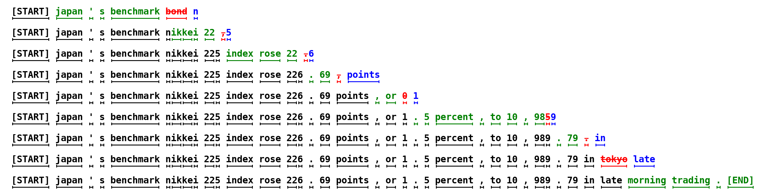
Figure 1: Each row is one iteration of the algorithm. Green tokens are draft suggestions from the small model that the large model accepted. Red tokens are rejected drafts. Blue tokens are corrections sampled from the adjusted distribution. In the first row, the large model ran once and 5 tokens were produced. The entire 38-token sentence required only 9 serial runs of the large model instead of 38.
Let’s trace one full iteration with \(\gamma = 3\), vocabulary {A, B, C, D}, and prefix = [The].
Stage 1 – Draft (\(M_q\) generates 3 tokens):
Stage 2 – Verify (\(M_p\) evaluates 4 positions in one batched call):
Stage 3 – Accept/Reject:
So \(n = 2\) (positions 1 and 2 accepted, position 3 rejected).
Compute the adjusted distribution at position 3:
\[p'(x) = \text{norm}(\max(0, p_3(x) - q_3(x)))\] \[= \text{norm}(\max(0, [0.1-0.2,\ 0.1-0.2,\ 0.1-0.3,\ 0.7-0.3]))\] \[= \text{norm}([0, 0, 0, 0.4]) = [0, 0, 0, 1.0]\]
Sample \(t =\) D from \(p'\).
Output: prefix + [A, B, D] = [The, A, B, D]. Three new tokens from one batched \(M_p\) call.
Recall: What are the three stages of speculative decoding? What happens when all \(\gamma\) draft tokens are accepted?
Apply: Given \(\gamma = 2\), draft tokens \(x_1 =\) B, \(x_2 =\) A, draft distributions \(q_1 = [0.2, 0.5, 0.3]\) and \(q_2 = [0.6, 0.3, 0.1]\), target distributions \(p_1 = [0.3, 0.4, 0.3]\) and \(p_2 = [0.4, 0.4, 0.2]\) and \(p_3 = [0.5, 0.3, 0.2]\), and random draws \(r_1 = 0.6\) and \(r_2 = 0.5\): determine \(n\), the output tokens, and the distribution used to sample the correction token.
Extend: The paper states that the verification step can batch \(\gamma + 1\) forward passes of \(M_p\) into a single call. Why is this possible? Consider what information each position needs – does position \(i\)’s computation depend on the result of position \(i-1\)’s computation during verification?
How well does the draft model match the target model? The acceptance rate \(\alpha\) quantifies this, and it connects to a natural measure of distribution overlap.
Imagine overlaying two bar charts – one for the target distribution \(p\) and one for the proposal distribution \(q\). The acceptance rate equals the total area of overlap between the two charts. Where the bars agree, proposals are always accepted. Where they disagree, some proposals are rejected.
The paper defines a divergence measure \(D_{LK}\):
\[D_{LK}(p, q) = \sum_x |p(x) - M(x)| = \sum_x |q(x) - M(x)|\]
where:
A key lemma connects this to the minimum function:
\[D_{LK}(p, q) = 1 - \sum_x \min(p(x), q(x))\]
This follows because \(\min(p, q) = \frac{p + q - |p - q|}{2}\), so \(\sum_x \min(p(x), q(x)) = \sum_x \frac{p + q - |p - q|}{2} = 1 - \sum_x \frac{|p - q|}{2} = 1 - D_{LK}(p, q)\).
The acceptance rate for a single prefix \(x_{<t}\) is:
\[\beta = \sum_x \min(p(x), q(x))\]
This is proved by computing the expected acceptance probability when sampling from \(q\):
\[\beta = E_{x \sim q(x)}\left[\min\left(1, \frac{p(x)}{q(x)}\right)\right] = \sum_x q(x) \cdot \min\left(1, \frac{p(x)}{q(x)}\right) = \sum_x \min(p(x), q(x))\]
The overall acceptance rate \(\alpha\) averages over all prefixes encountered during generation:
\[\alpha = E(\beta) = E\left(\sum_x \min(p(x), q(x))\right)\]
Properties of \(D_{LK}\):
Let’s compute \(\alpha\) for a small example with two prefixes.
Prefix 1: \(p = [0.5, 0.3, 0.2]\), \(q = [0.3, 0.4, 0.3]\).
\[\beta_1 = \min(0.5, 0.3) + \min(0.3, 0.4) + \min(0.2, 0.3) = 0.3 + 0.3 + 0.2 = 0.8\]
Prefix 2: \(p = [0.7, 0.2, 0.1]\), \(q = [0.1, 0.6, 0.3]\).
\[\beta_2 = \min(0.7, 0.1) + \min(0.2, 0.6) + \min(0.1, 0.3) = 0.1 + 0.2 + 0.1 = 0.4\]
Assuming both prefixes are equally likely, the average:
\[\alpha = E(\beta) = \frac{0.8 + 0.4}{2} = 0.6\]
Notice how prefix 2 has much lower overlap – the two models strongly disagree about the next token. This lowers the overall \(\alpha\). In practice, \(\alpha\) varies between 0.5 and 0.9 for approximation models that are about 100x smaller than the target.
Also notice: argmax (temperature=0) produces sharper distributions. If both models agree on the top token, \(\min(p, q)\) is high because most mass concentrates there. This is why the paper observes higher \(\alpha\) values for argmax sampling than for temperature=1 sampling.
Recall: What does \(\beta = \sum_x \min(p(x), q(x))\) measure geometrically? What happens to \(\beta\) when \(p = q\)?
Apply: Given \(p = [0.8, 0.1, 0.05, 0.05]\) and \(q = [0.7, 0.15, 0.1, 0.05]\), compute \(\beta\) and \(D_{LK}(p, q)\). Then compute \(\beta\) for the same distributions after argmax standardization (zero out all non-maximum elements and renormalize).
Extend: The paper reports that even a trivial bigram model achieves \(\alpha \approx 0.2\) when used with T5-XXL. Why would a bigram model (which only looks at the previous token to predict the next one) have any overlap with a sophisticated 11-billion-parameter model? What does this tell you about the structure of language?
The final piece of the puzzle: how do acceptance rate, draft cost, and speculation depth combine to determine the actual walltime improvement? This lesson derives the speedup formula and identifies when speculative decoding is guaranteed to help.
Think about a factory assembly line. The standard process takes 1 hour per unit (one \(M_p\) forward pass per token). A speculative process uses a fast pre-checker (costing \(c\) hours per check) to draft \(\gamma\) units, then verifies all of them in one 1-hour quality pass. If the expected acceptance rate is \(\alpha\), the expected number of good units per quality pass is \(\frac{1 - \alpha^{\gamma+1}}{1 - \alpha}\). The speedup is the ratio of tokens produced to total time spent.
The expected number of tokens per iteration follows a capped geometric distribution:
\[E(\#\ \text{generated tokens}) = \frac{1 - \alpha^{\gamma + 1}}{1 - \alpha}\]
where:
This formula arises because: with probability \(\alpha^{\gamma}\) all \(\gamma\) drafts are accepted and we get \(\gamma + 1\) tokens. With probability \((1-\alpha)\alpha^{k}\) for \(k = 0, 1, \ldots, \gamma-1\), exactly \(k\) drafts are accepted before the first rejection, giving \(k+1\) tokens. Summing: \(\sum_{k=0}^{\gamma-1}(k+1)(1-\alpha)\alpha^k + (\gamma+1)\alpha^{\gamma} = \frac{1 - \alpha^{\gamma+1}}{1 - \alpha}\).
Each iteration costs \(\gamma c + 1\) units of \(M_p\) runtime (\(\gamma\) runs of \(M_q\) at cost \(c\) each, plus one batched run of \(M_p\)). The walltime speedup factor is:
\[\text{Speedup} = \frac{1 - \alpha^{\gamma + 1}}{(1 - \alpha)(\gamma c + 1)}\]
where:
When \(c \approx 0\) (draft model has negligible cost), the speedup equals the expected tokens per iteration. When \(c > 0\), the denominator penalizes larger \(\gamma\) because more drafts cost more time.
The minimum viability condition (Corollary 3.9) states:
\[\alpha > c \implies \exists\ \gamma : \text{Speedup} > 1\]
Evaluating the speedup formula at \(\gamma = 1\):
\[\text{Speedup}|_{\gamma=1} = \frac{1 - \alpha^2}{(1 - \alpha)(c + 1)} = \frac{1 + \alpha}{1 + c}\]
If \(\alpha > c\), then \(\frac{1 + \alpha}{1 + c} > 1\). Since \(c\) is typically below 0.05 and \(\alpha\) is typically above 0.5, this condition is satisfied in virtually all practical scenarios. Even a bigram model (\(\alpha \approx 0.2\), \(c \approx 0\)) yields a \(\frac{1.2}{1.0} = 1.2\)x speedup.
The optimal \(\gamma\) depends on \(\alpha\) and \(c\). Higher \(\alpha\) justifies larger \(\gamma\) (more drafts will be accepted). Higher \(c\) favors smaller \(\gamma\) (drafts are expensive). In the paper’s experiments, optimal \(\gamma\) ranges from 3 to 10.
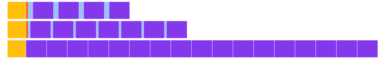
Figure 5: A simplified execution trace for an encoder-decoder Transformer. Top: speculative decoding with gamma=7. Middle: gamma=3. Bottom: standard decoding. Speculative decoding completes in fewer large-model calls, reducing total walltime despite more total computation.
Let’s compute the speedup for the paper’s best T5-XXL configuration.
Given: \(\alpha = 0.75\), \(\gamma = 7\), \(c = 0.02\).
Expected tokens per iteration:
\[E = \frac{1 - 0.75^{8}}{1 - 0.75} = \frac{1 - 0.100}{0.25} = \frac{0.900}{0.25} = 3.60\]
Walltime cost per iteration (in units of one \(M_p\) forward pass):
\[\text{cost} = \gamma c + 1 = 7 \times 0.02 + 1 = 0.14 + 1 = 1.14\]
Speedup:
\[\text{Speedup} = \frac{3.60}{1.14} = 3.16\text{x}\]
The paper measured 3.4x empirically – reasonably close to the theoretical prediction. The small discrepancy comes from implementation details and the simplifying i.i.d. (independent and identically distributed – each acceptance decision has the same probability and does not depend on previous decisions) assumption.
Now let’s check the minimum viability condition. Is \(\alpha > c\)? Yes: \(0.75 > 0.02\). The guaranteed minimum speedup at \(\gamma = 1\) is:
\[\frac{1 + 0.75}{1 + 0.02} = \frac{1.75}{1.02} = 1.72\text{x}\]
Even with just one draft token, we get a 1.72x speedup.
Comparison with a larger draft model: T5-large (\(\alpha = 0.82\), \(c = 0.11\), \(\gamma = 7\)):
\[\text{Speedup} = \frac{1 - 0.82^{8}}{(1 - 0.82)(7 \times 0.11 + 1)} = \frac{1 - 0.204}{0.18 \times 1.77} = \frac{0.796}{0.319} = 2.50\text{x}\]
The paper measured 1.7x. Despite higher \(\alpha\), the larger draft model’s higher cost (\(c = 0.11\) vs. \(c = 0.02\)) reduces the speedup. The smallest model wins because its negligible cost outweighs its lower acceptance rate.
Recall: Write out the speedup formula and explain what each variable represents. Under what condition is speculative decoding guaranteed to provide a speedup?
Apply: A system uses a 1B-parameter draft model (\(c = 0.03\)) with a 70B-parameter target model. The measured acceptance rate is \(\alpha = 0.7\) with \(\gamma = 5\). Compute the expected tokens per iteration, the walltime cost per iteration, and the speedup factor. Then compute the speedup at \(\gamma = 10\) and determine which \(\gamma\) is better.
Extend: The paper mentions that an “oracle” that adaptively chooses \(\gamma\) for each position could improve the speedup by up to 60%. Why would adaptive \(\gamma\) help? Consider a sequence where some tokens are very predictable (high \(\beta\)) and others are surprising (low \(\beta\)). What would the oracle do differently at each position?
Speculative decoding guarantees that the output distribution is identical to the target model alone. Walk through the mathematical argument for why this is true – specifically, how do the acceptance and rejection terms combine to give \(P(x = x') = p(x')\)?
The paper finds that the smallest approximation model (T5-small, 77M parameters) gives the best speedup despite having a lower acceptance rate than larger approximation models. Explain this counterintuitive result using the speedup formula. What is the optimal balance between \(\alpha\) and \(c\)?
How does speculative decoding relate to BERT’s (see BERT) ability to process all tokens in parallel? In what sense does speculative decoding recover some of BERT’s parallelism for autoregressive models?
What are the main scenarios where speculative decoding would NOT help? Consider hardware utilization, batch sizes, and the relationship between compute and memory bandwidth.
Chain-of-thought prompting (see Chain-of-Thought Prompting) and Tree of Thoughts (see Tree of Thoughts) improve output quality at the cost of generating more tokens. Speculative decoding reduces the cost of generating tokens without changing quality. How might these techniques combine? Would speculative decoding be more or less effective when generating chain-of-thought reasoning?
Build a numpy simulation of speculative decoding that demonstrates the algorithm’s behavior, measures acceptance rates, computes expected speedups, and verifies that the output distribution matches the target model.
You will implement:
Both “models” are simulated as functions that return probability distributions given a prefix. No real neural networks are needed.
import numpy as np


def speculative_sample(p, q, rng):
    """
    Sample a single token from target distribution p using proposal
    distribution q via speculative sampling.

    Algorithm:
    1. Sample x from q.
    2. With probability min(1, p[x]/q[x]), accept x.
    3. If rejected, sample from the adjusted distribution
       p'(x) = norm(max(0, p(x) - q(x))).

    Args:
        p: numpy array, target distribution (sums to 1)
        q: numpy array, proposal distribution (sums to 1)
        rng: numpy random generator

    Returns:
        (token_index, accepted): the sampled token and whether the
        proposal was accepted (True) or a correction was drawn (False)
    """
    # TODO: implement
    pass


def compute_acceptance_rate(p, q):
    """
    Compute the theoretical acceptance rate beta = sum_x min(p(x), q(x)).

    Args:
        p: numpy array, target distribution
        q: numpy array, proposal distribution

    Returns:
        float: the acceptance rate beta
    """
    # TODO: implement
    pass


def speculative_decoding_step(target_model, draft_model, prefix, gamma, rng):
    """
    Run one iteration of the speculative decoding algorithm.

    Stage 1 - Draft: generate gamma tokens from draft_model autoregressively.
    Stage 2 - Verify: get target_model distributions for all gamma+1 positions.
    Stage 3 - Accept/Reject: use speculative sampling to determine how many
              draft tokens to accept, then sample a correction/bonus token.

    Args:
        target_model: function(prefix) -> probability distribution over vocab
        draft_model: function(prefix) -> probability distribution over vocab
        prefix: list of token indices generated so far
        gamma: number of draft tokens to generate
        rng: numpy random generator

    Returns:
        new_tokens: list of token indices produced in this iteration (1 to gamma+1)
    """
    # TODO: implement
    pass


def verify_distribution(target_dist, proposal_dist, rng, n_samples=100000):
    """
    Verify that speculative sampling produces the target distribution.
    Generate n_samples tokens via speculative_sample and compare the
    empirical frequencies to the target distribution.

    Args:
        target_dist: numpy array, target distribution
        proposal_dist: numpy array, proposal distribution
        rng: numpy random generator
        n_samples: number of samples to draw

    Returns:
        (empirical_dist, max_absolute_error): the observed frequencies
        and the maximum deviation from the target
    """
    # TODO: implement
    pass


def compute_speedup(alpha, gamma, c):
    """
    Compute the theoretical walltime speedup factor.

    Speedup = (1 - alpha^(gamma+1)) / ((1 - alpha) * (gamma * c + 1))

    Args:
        alpha: expected acceptance rate
        gamma: number of draft tokens
        c: cost coefficient (ratio of draft model time to target model time)

    Returns:
        float: the speedup factor
    """
    # TODO: implement
    pass


def simulate_speedup(target_model, draft_model, prefix, gamma, c,
                     n_iterations, rng):
    """
    Simulate many iterations of speculative decoding and compute the
    empirical speedup.

    For each iteration:
    - Run speculative_decoding_step to get new_tokens
    - The walltime cost is (gamma * c + 1) per iteration
    - The tokens produced is len(new_tokens) per iteration

    Speedup = total_tokens / total_cost (compared to 1 token per cost 1).

    Args:
        target_model: function(prefix) -> probability distribution
        draft_model: function(prefix) -> probability distribution
        prefix: initial prefix
        gamma: number of draft tokens
        c: cost coefficient
        n_iterations: number of iterations to simulate
        rng: numpy random generator

    Returns:
        (empirical_speedup, avg_tokens_per_iter, avg_acceptance_rate)
    """
    # TODO: implement
    pass


def run_experiment():
    """Run the full speculative decoding experiment."""
    rng = np.random.default_rng(42)
    vocab_size = 8

    # --- Experiment 1: Verify distribution correctness ---
    print("Experiment 1: Distribution Verification")
    print("=" * 55)
    p = np.array([0.35, 0.25, 0.15, 0.10, 0.07, 0.04, 0.02, 0.02])
    q = np.array([0.20, 0.20, 0.20, 0.15, 0.10, 0.08, 0.05, 0.02])

    beta = compute_acceptance_rate(p, q)
    print(f"Target:   {p}")
    print(f"Proposal: {q}")
    print(f"Acceptance rate (beta): {beta:.3f}")

    empirical, max_err = verify_distribution(p, q, rng)
    print(f"Empirical: {np.round(empirical, 3)}")
    print(f"Max absolute error: {max_err:.4f}")
    print(f"Distribution match: {'PASS' if max_err < 0.01 else 'FAIL'}")
    print()

    # --- Experiment 2: Theoretical speedup across configurations ---
    print("Experiment 2: Theoretical Speedup")
    print("=" * 55)
    print(f"{'alpha':<8}{'gamma':<8}{'c':<8}{'Tokens/iter':<14}{'Speedup':<10}")
    print("-" * 55)

    configs = [
        (0.5, 3, 0.02),
        (0.7, 5, 0.02),
        (0.75, 7, 0.02),   # paper's T5-small config
        (0.8, 7, 0.04),    # paper's T5-base config
        (0.82, 7, 0.11),   # paper's T5-large config
        (0.9, 10, 0.02),
    ]
    for alpha, gamma, c in configs:
        tokens = (1 - alpha ** (gamma + 1)) / (1 - alpha)
        speedup = compute_speedup(alpha, gamma, c)
        print(f"{alpha:<8}{gamma:<8}{c:<8}{tokens:<14.2f}{speedup:<10.2f}x")
    print()

    # --- Experiment 3: Simulated speculative decoding ---
    print("Experiment 3: Simulated Speculative Decoding")
    print("=" * 55)

    # Simple "models": target is sharper, draft is flatter
    def target_model(prefix):
        # Deterministic distribution that depends mildly on prefix length
        base = np.array([0.40, 0.25, 0.15, 0.08, 0.05, 0.03, 0.02, 0.02])
        shift = len(prefix) % vocab_size
        return np.roll(base, shift)

    def draft_model(prefix):
        # Flatter version of target -- less confident but roughly aligned
        base = np.array([0.25, 0.20, 0.18, 0.12, 0.10, 0.07, 0.05, 0.03])
        shift = len(prefix) % vocab_size
        return np.roll(base, shift)

    for gamma in [3, 5, 7]:
        c = 0.02
        emp_speedup, avg_tokens, avg_alpha = simulate_speedup(
            target_model, draft_model, prefix=[0], gamma=gamma,
            c=c, n_iterations=1000, rng=rng
        )
        theo_speedup = compute_speedup(avg_alpha, gamma, c)
        print(f"gamma={gamma}: avg_tokens/iter={avg_tokens:.2f}, "
              f"avg_alpha={avg_alpha:.2f}, "
              f"empirical={emp_speedup:.2f}x, "
              f"theoretical={theo_speedup:.2f}x")

    # --- Experiment 4: Minimum viability condition ---
    print()
    print("Experiment 4: Minimum Viability Condition")
    print("=" * 55)
    print(f"{'alpha':<8}{'c':<8}{'alpha > c?':<12}{'Min speedup':<14}")
    print("-" * 55)
    for alpha, c in [(0.1, 0.02), (0.3, 0.05), (0.5, 0.02),
                     (0.75, 0.02), (0.02, 0.05)]:
        viable = alpha > c
        min_speedup = (1 + alpha) / (1 + c) if viable else 0.0
        print(f"{alpha:<8}{c:<8}{'Yes' if viable else 'No':<12}"
              f"{min_speedup:<14.2f}x" if viable else
              f"{alpha:<8}{c:<8}{'No':<12}{'N/A':<14}")


if __name__ == "__main__":
run_experiment()Experiment 1: Distribution Verification
=======================================================
Target: [0.35 0.25 0.15 0.1 0.07 0.04 0.02 0.02]
Proposal: [0.2 0.2 0.2 0.15 0.1 0.08 0.05 0.02]
Acceptance rate (beta): 0.780
Empirical: [0.351 0.249 0.149 0.101 0.07 0.04 0.02 0.02 ]
Max absolute error: 0.0025
Distribution match: PASS
Experiment 2: Theoretical Speedup
=======================================================
alpha gamma c Tokens/iter Speedup
-------------------------------------------------------
0.5 3 0.02 1.88 1.77x
0.7 5 0.02 2.88 2.62x
0.75 7 0.02 3.60 3.16x
0.8 7 0.04 4.40 3.33x
0.82 7 0.11 4.76 2.50x
0.9 10 0.02 6.86 5.72x
Experiment 3: Simulated Speculative Decoding
=======================================================
gamma=3: avg_tokens/iter=2.68, avg_alpha=0.72, empirical=2.53x, theoretical=2.48x
gamma=5: avg_tokens/iter=3.31, avg_alpha=0.72, empirical=2.99x, theoretical=2.89x
gamma=7: avg_tokens/iter=3.62, avg_alpha=0.72, empirical=3.13x, theoretical=3.09x
Experiment 4: Minimum Viability Condition
=======================================================
alpha c alpha > c? Min speedup
-------------------------------------------------------
0.1 0.02 Yes 1.08x
0.3 0.05 Yes 1.24x
0.5 0.02 Yes 1.47x
0.75 0.02 Yes 1.72x
0.02 0.05 No N/AThe exact numbers will vary with the random seed, but the patterns should be clear: (1) speculative sampling produces the correct target distribution, (2) theoretical and empirical speedups closely match, (3) increasing \(\gamma\) gives diminishing returns, and (4) the minimum viability condition \(\alpha > c\) correctly predicts when speculative decoding helps.