By the end of this course, you will be able to:
Before the Transformer, the best language models processed words one at a time, left to right. This lesson explains why that’s a problem and what it costs.
Imagine translating a book from English to French by reading one word at a time, trying to keep everything in your head. You read “The,” update your mental notes. Then “cat,” update again. Then “sat.” By word 50, you’ve partially forgotten what word 1 said. And you can’t read word 5 until you’ve finished processing word 4 – there’s no way to skip ahead and work in parallel.
This is how a recurrent neural network (RNN) works. An RNN processes a sequence of tokens (words, subwords, or characters) one position at a time. At each position \(t\), it computes a hidden state \(h_t\) as a function of the previous hidden state \(h_{t-1}\) and the current input \(x_t\):
\[h_t = f(h_{t-1}, x_t)\]
This creates two problems:
Problem 1: No parallelism. Computing \(h_5\) requires \(h_4\), which requires \(h_3\), and so on. On a GPU (hardware designed to do thousands of operations simultaneously), most of the chip sits idle while the RNN processes one position at a time. Training a large model on millions of sentences becomes painfully slow.
Problem 2: Long-range dependencies decay. Information from word 1 must survive a chain of \(n\) transformations to reach word \(n\). In practice, signals degrade across long chains – like a game of telephone. If the verb at position 40 needs to agree with the subject at position 3, the model struggles because the relevant information has been diluted through 37 sequential steps.
A technique called attention was invented to help with problem 2. It lets the model look directly at any previous position, creating a shortcut: instead of passing information through 37 steps, the model reaches back and reads position 3 directly. But before this paper, attention was always used as an addition to RNNs – the sequential backbone remained.
The Transformer’s radical idea: throw away the RNN entirely. Use attention as the only mechanism for relating positions in the sequence. Every position looks at every other position in a single step. The maximum path length between any two positions drops from \(O(n)\) to \(O(1)\) – a constant, regardless of sequence length. And since every position is processed simultaneously, the entire computation is parallelizable.
Consider a 5-word sentence: [“I”, “love”, “deep”, “learning”, “models”].
RNN processing (sequential):
Total: 5 sequential steps. If each step takes 1 ms, the sequence takes 5 ms.
For “models” to know about “I”, information passes through: \(h_1 \to h_2 \to h_3 \to h_4 \to h_5\). Path length: 4 hops.
Transformer processing (parallel):
Total: 1 step. “models” directly attends to “I” in a single operation. Path length: 1 hop.
On a GPU with 5000 cores, the Transformer uses 5 cores in parallel for 1 step. The RNN uses 1 core for 5 steps. As sentences get longer (100, 1000 words), the Transformer’s advantage grows dramatically.
Recall: What are the two main problems with RNNs that the Transformer addresses? Which one is about speed and which is about quality?
Apply: A sentence has 100 words. How many sequential steps does an RNN need? How many does the Transformer need? What’s the maximum path length between word 1 and word 100 in each model?
Extend: The Transformer’s self-attention has \(O(n^2 \cdot d)\) computation per layer (where \(n\) is sequence length and \(d\) is embedding dimension), while an RNN layer has \(O(n \cdot d^2)\). For what relationship between \(n\) and \(d\) is the Transformer more efficient? In typical language models, \(d = 512\) and \(n\) ranges from 50 to 512 – which regime are we in?
Attention works by measuring how relevant each word is to every other word. The Transformer measures relevance using dot products. This lesson builds the mathematical intuition for why dot products measure similarity.
Think of two arrows pointing in the same direction. They agree – they’re similar. Two arrows pointing in opposite directions disagree – they’re dissimilar. Two arrows at right angles are unrelated. The dot product captures exactly this intuition.
For two vectors \(a = [a_1, a_2, \ldots, a_d]\) and \(b = [b_1, b_2, \ldots, b_d]\):
\[a \cdot b = \sum_{i=1}^{d} a_i b_i = \|a\| \|b\| \cos \theta\]
The dot product is large and positive when vectors are similar, near zero when unrelated, and large and negative when opposite.
When we compute dot products for an entire sequence at once, we use matrix multiplication. If we have \(n\) query vectors (each of dimension \(d\)) packed into a matrix \(Q\) of shape \((n \times d)\), and \(m\) key vectors packed into a matrix \(K\) of shape \((m \times d)\), then:
\[QK^T\]
produces an \((n \times m)\) matrix where entry \((i, j)\) is the dot product between query \(i\) and key \(j\). Every pair of (query, key) gets a similarity score in a single matrix multiplication – exactly the kind of operation GPUs excel at.
Let’s compute similarity between 3 words using 2-dimensional vectors.
Suppose our word vectors are:
Pack them into \(Q = K = \begin{bmatrix} 1.0 & 0.5 \\ 0.9 & 0.6 \\ -0.3 & 0.8 \end{bmatrix}\)
Compute \(QK^T\):
Row 1 (cat) vs all:
Row 2 (dog) vs all:
Row 3 (car) vs all:
\[QK^T = \begin{bmatrix} 1.25 & 1.20 & 0.10 \\ 1.20 & 1.17 & 0.21 \\ 0.10 & 0.21 & 0.73 \end{bmatrix}\]
Reading the first row: “cat” is most similar to itself (1.25), almost as similar to “dog” (1.20), and barely related to “car” (0.10). This matches our intuition – cats and dogs are both animals, while cars are something else entirely.
Recall: Why does the Transformer use dot products rather than, say, Euclidean distance to measure similarity between words? (Hint: think about computational efficiency with matrix multiplication.)
Apply: Compute the dot product between \(a = [2, -1, 3]\) and \(b = [1, 4, -2]\). Are these vectors more similar or dissimilar? How would you interpret the sign of the result?
Extend: If \(q\) and \(k\) are \(d_k\)-dimensional vectors whose components are independent random variables with mean 0 and variance 1, the expected value of their dot product is 0 and its variance is \(d_k\). Show why: compute \(\text{Var}(q \cdot k) = \text{Var}(\sum_{i=1}^{d_k} q_i k_i)\). What does this imply about the magnitude of dot products when \(d_k = 512\) vs. \(d_k = 4\)?
This lesson introduces the Transformer’s core computation: the attention mechanism that lets every word look at every other word and decide what’s relevant.
Imagine you’re writing a book report and have the full text spread on a desk. For each sentence you write, you scan all parts of the book and focus on the most relevant passages. Some passages get most of your attention (you read them carefully), others get a quick glance, and most you ignore entirely. The amount of attention each passage gets depends on how relevant it is to what you’re currently writing.
Scaled dot-product attention formalizes this. Each position in the sequence produces three vectors from its input:
The queries, keys, and values are computed by multiplying the input by learned weight matrices. When we process all positions at once, we get matrices \(Q\), \(K\), and \(V\). The attention output is:
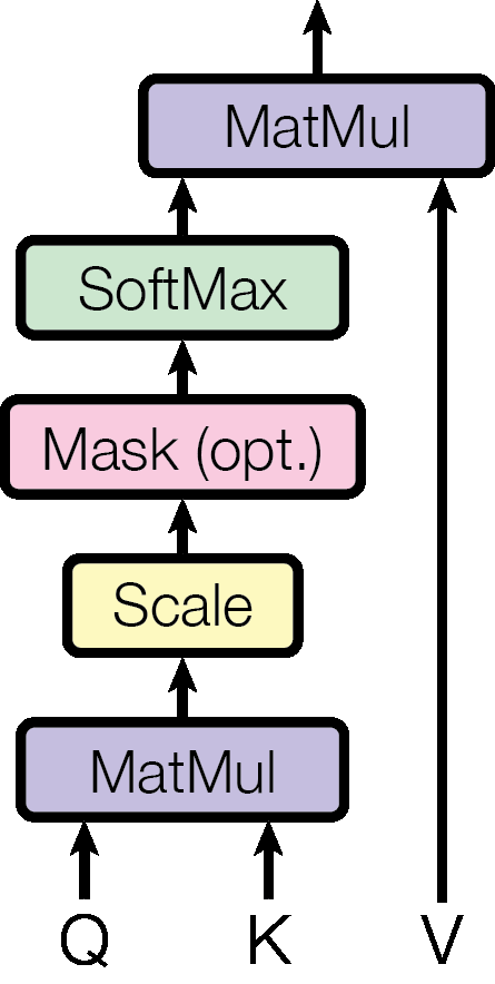
\[\text{Attention}(Q, K, V) = \text{softmax}\left(\frac{QK^T}{\sqrt{d_k}}\right)V\]
Why scale by \(\sqrt{d_k}\)? When \(d_k\) is large, dot products tend to have large magnitudes. If the components of \(q\) and \(k\) are independent random variables with mean 0 and variance 1, their dot product has mean 0 and variance \(d_k\). With \(d_k = 64\), dot products can easily reach values like \(\pm 8\). When you feed large values into softmax, it saturates – it pushes almost all the probability mass onto one position, producing near-zero gradients everywhere else. Dividing by \(\sqrt{d_k}\) normalizes the variance back to 1, keeping the softmax in a region where gradients flow and the model can learn.
Figure 1: Scaled Dot-Product Attention. Queries and Keys are multiplied (MatMul), scaled by \(1/\sqrt{d_k}\), optionally masked (to block future positions in the decoder), passed through softmax to get attention weights, then multiplied with Values to produce the output.
The algorithm, step by step:
Let our input be the 3-word sentence [“the”, “cat”, “sat”] with \(d_k = d_v = 2\) (tiny dimensions for hand computation).
After multiplying by learned weight matrices, suppose we get:
\[Q = \begin{bmatrix} 1 & 0 \\ 0 & 1 \\ 1 & 1 \end{bmatrix}, \quad K = \begin{bmatrix} 1 & 0 \\ 0 & 1 \\ 0.5 & 0.5 \end{bmatrix}, \quad V = \begin{bmatrix} 0.1 & 0.9 \\ 0.8 & 0.2 \\ 0.5 & 0.5 \end{bmatrix}\]
Step 1: Score. \(QK^T\):
| key: “the” | key: “cat” | key: “sat” | |
|---|---|---|---|
| query: “the” | \(1 \times 1 + 0 \times 0 = 1.0\) | \(1 \times 0 + 0 \times 1 = 0.0\) | \(1 \times 0.5 + 0 \times 0.5 = 0.5\) |
| query: “cat” | \(0 \times 1 + 1 \times 0 = 0.0\) | \(0 \times 0 + 1 \times 1 = 1.0\) | \(0 \times 0.5 + 1 \times 0.5 = 0.5\) |
| query: “sat” | \(1 \times 1 + 1 \times 0 = 1.0\) | \(1 \times 0 + 1 \times 1 = 1.0\) | \(1 \times 0.5 + 1 \times 0.5 = 1.0\) |
\[QK^T = \begin{bmatrix} 1.0 & 0.0 & 0.5 \\ 0.0 & 1.0 & 0.5 \\ 1.0 & 1.0 & 1.0 \end{bmatrix}\]
Step 2: Scale. Divide by \(\sqrt{d_k} = \sqrt{2} \approx 1.414\):
\[\frac{QK^T}{\sqrt{2}} = \begin{bmatrix} 0.707 & 0.000 & 0.354 \\ 0.000 & 0.707 & 0.354 \\ 0.707 & 0.707 & 0.707 \end{bmatrix}\]
Step 3: Softmax (row-wise). For row 1: \(\text{softmax}([0.707, 0.000, 0.354])\)
For row 2: \(\text{softmax}([0.000, 0.707, 0.354])\)
For row 3: \(\text{softmax}([0.707, 0.707, 0.707])\)
\[\text{Weights} = \begin{bmatrix} 0.456 & 0.225 & 0.320 \\ 0.225 & 0.456 & 0.320 \\ 0.333 & 0.333 & 0.333 \end{bmatrix}\]
Step 4: Aggregate. Multiply weights by \(V\):
Output row 1 (“the”): \(0.456 \times [0.1, 0.9] + 0.225 \times [0.8, 0.2] + 0.320 \times [0.5, 0.5]\) \(= [0.046, 0.410] + [0.180, 0.045] + [0.160, 0.160] = [0.386, 0.615]\)
Output row 2 (“cat”): \(0.225 \times [0.1, 0.9] + 0.456 \times [0.8, 0.2] + 0.320 \times [0.5, 0.5]\) \(= [0.023, 0.203] + [0.365, 0.091] + [0.160, 0.160] = [0.547, 0.454]\)
Output row 3 (“sat”): \(0.333 \times [0.1, 0.9] + 0.333 \times [0.8, 0.2] + 0.333 \times [0.5, 0.5]\) \(= [0.033, 0.300] + [0.267, 0.067] + [0.167, 0.167] = [0.467, 0.533]\)
The output for “the” is heavily influenced by its own value (weight 0.456) with contributions from “sat” (0.320) and “cat” (0.225). The word “sat” attends equally to all three words (all scores were the same after scaling). Each output is a context-aware representation that blends information from the entire sequence.
Recall: What happens to the attention weights if you remove the \(\sqrt{d_k}\) scaling factor and \(d_k\) is large? Why is this a problem for learning?
Apply: Given \(Q = \begin{bmatrix} 1 & 0 \end{bmatrix}\), \(K = \begin{bmatrix} 1 & 0 \\ 0 & 1 \end{bmatrix}\), \(V = \begin{bmatrix} 5 \\ 3 \end{bmatrix}\) with \(d_k = 2\), compute \(\text{Attention}(Q, K, V)\). Show each step: score, scale, softmax, aggregate.
Extend: In the decoder, a mask is applied before softmax to prevent each position from attending to future positions. If the mask sets score \((i, j)\) to \(-\infty\) for all \(j > i\), what do the attention weights look like for a 4-word sequence? Draw the weight matrix (which entries are zero, which are non-zero). Why is this masking necessary for generating text one word at a time?
A single attention head captures one type of relationship. Multi-head attention runs several attention heads in parallel, each learning to focus on different aspects of the input. This is one of the paper’s key architectural choices.
Imagine you’re analyzing a sentence: “The animal didn’t cross the street because it was too tired.” To understand “it,” you need to consider multiple types of relationships simultaneously:
A single attention head computes one set of attention weights – it can only focus on one pattern at a time. Multi-head attention solves this by running \(h\) independent attention heads, each projecting the input into a different subspace where it learns to capture different relationships.
\[\text{MultiHead}(Q, K, V) = \text{Concat}(\text{head}_1, \ldots, \text{head}_h)W^O\]
\[\text{where } \text{head}_i = \text{Attention}(QW^Q_i, KW^K_i, VW^V_i)\]
The key insight: instead of running one attention function on 512-dimensional vectors, we run 8 attention functions on 64-dimensional vectors. Each head independently learns what to attend to. The concatenated output (8 heads × 64 dimensions = 512 dimensions) is projected through \(W^O\) to produce the final 512-dimensional output.
The total computation is similar to a single attention head at full dimension, because each head operates on smaller vectors. But the model’s capacity is much greater – it can simultaneously capture multiple types of relationships.
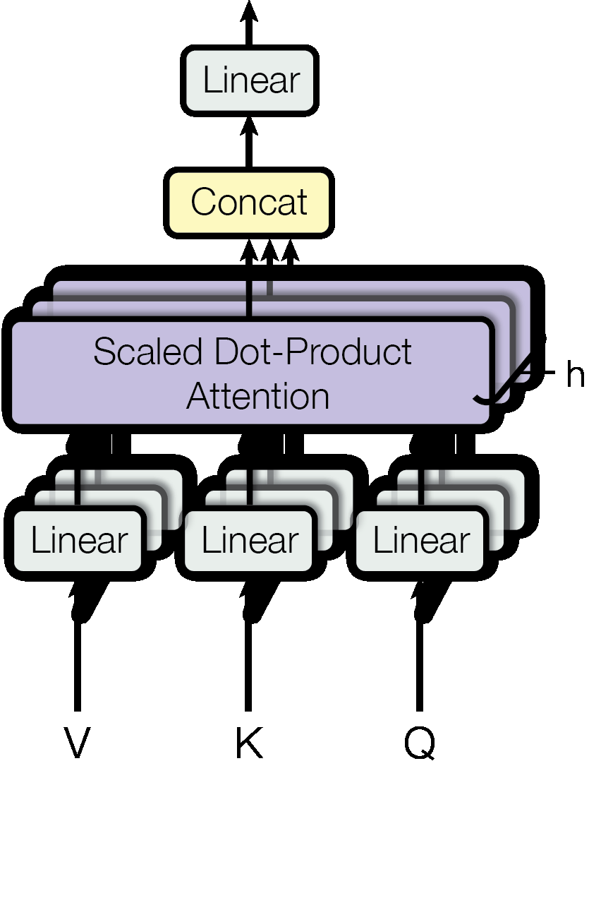
Figure 2: Multi-Head Attention. Inputs V, K, Q are each projected through \(h\) separate learned linear transformations, producing \(h\) sets of lower-dimensional queries, keys, and values. Scaled dot-product attention runs on each set in parallel, the results are concatenated, and a final linear layer maps back to the original dimension.
Let’s trace multi-head attention with \(h = 2\) heads, \(d_\text{model} = 4\), \(d_k = d_v = 2\).
Our input is a 2-word sequence with 4-dimensional embeddings:
\[X = \begin{bmatrix} 1.0 & 0.5 & -0.5 & 0.2 \\ 0.3 & -0.1 & 0.8 & 0.6 \end{bmatrix}\]
For self-attention, \(Q = K = V = X\).
Head 1 projections (project from 4D to 2D):
\[W^Q_1 = \begin{bmatrix} 0.5 & 0.1 \\ -0.2 & 0.4 \\ 0.3 & -0.1 \\ 0.1 & 0.3 \end{bmatrix}, \quad W^K_1 = \begin{bmatrix} 0.3 & -0.2 \\ 0.1 & 0.5 \\ -0.1 & 0.2 \\ 0.4 & 0.1 \end{bmatrix}\]
Compute projected queries for head 1: \(Q_1 = XW^Q_1\)
Row 1: \(1.0(0.5) + 0.5(-0.2) + (-0.5)(0.3) + 0.2(0.1) = 0.27\), \(1.0(0.1) + 0.5(0.4) + (-0.5)(-0.1) + 0.2(0.3) = 0.41\)
Row 2: \(0.3(0.5) + (-0.1)(-0.2) + 0.8(0.3) + 0.6(0.1) = 0.47\), \(0.3(0.1) + (-0.1)(0.4) + 0.8(-0.1) + 0.6(0.3) = 0.07\)
\[Q_1 = \begin{bmatrix} 0.27 & 0.41 \\ 0.47 & 0.07 \end{bmatrix}\]
Similarly compute \(K_1 = XW^K_1\) and \(V_1 = XW^V_1\) (using their respective projection matrices).
Then apply scaled dot-product attention on these 2D projected vectors: \(\text{head}_1 = \text{Attention}(Q_1, K_1, V_1)\). This produces a \((2 \times 2)\) output.
Head 2 does the same thing with different projection matrices \(W^Q_2\), \(W^K_2\), \(W^V_2\), learning different relationships. This produces another \((2 \times 2)\) output.
Concatenate: \(\text{Concat}(\text{head}_1, \text{head}_2)\) has shape \((2 \times 4)\) – the two 2D outputs side by side.
Output projection: multiply by \(W^O\) (shape \(4 \times 4\)) to get the final \((2 \times 4)\) output.
The result: each word gets a new 4-dimensional representation that combines insights from both attention heads. Head 1 might have learned to attend to syntactic neighbors, while head 2 learned to attend to semantically related words.
Recall: Why does multi-head attention split the dimensions among heads (\(d_k = d_\text{model} / h\)) rather than giving each head the full \(d_\text{model}\) dimensions? What would happen to the computational cost if each head used full dimensions?
Apply: With \(d_\text{model} = 512\) and \(h = 8\), how many parameters are in the four projection matrices (\(W^Q_i\), \(W^K_i\), \(W^V_i\), \(W^O\)) for all heads combined? Count each matrix separately, then sum. (Ignore biases.)
Extend: The paper’s ablation study (Table 3, rows A) found that \(h = 1\) head performs 0.9 BLEU worse than \(h = 8\) heads, but \(h = 32\) heads also degrades. Why would too many heads hurt quality? Think about what happens to \(d_k\) as \(h\) increases.
The Transformer processes all positions in parallel – it sees the entire sequence at once. But this means it has no idea which word comes first, second, or last. Without positional information, “the cat sat on the mat” and “mat the on sat cat the” are identical. This lesson adds position awareness.
Think of sending a message where all the letters arrive at the same time in a jumbled pile. You need some way to mark each letter with its position so the recipient can put them in order. That’s what positional encoding does: it stamps each word with a signal that says “I’m in position \(pos\).”
The Transformer adds a positional encoding vector to each word’s embedding before feeding it into the model. The positional encoding \(PE\) has the same dimension as the word embedding (\(d_\text{model} = 512\)), so they can simply be added together:
\[\text{input}_i = \text{embedding}_i + PE_i\]
The paper uses sinusoidal functions to generate positional encodings:
\[PE_{(pos,2i)} = \sin\left(\frac{pos}{10000^{2i/d_\text{model}}}\right)\]
\[PE_{(pos,2i+1)} = \cos\left(\frac{pos}{10000^{2i/d_\text{model}}}\right)\]
Each dimension is a sinusoidal wave with a different frequency. Low dimensions oscillate rapidly (high frequency, short wavelength), distinguishing nearby positions. High dimensions oscillate slowly (low frequency, long wavelength), encoding coarser position information. Together, the full vector forms a unique “fingerprint” for each position.
Why sinusoids instead of learned position embeddings? The authors hypothesized that sinusoidal encodings would let the model generalize to sequence lengths longer than seen during training. The key mathematical property: for any fixed offset \(k\), the encoding \(PE_{pos+k}\) can be expressed as a linear function of \(PE_{pos}\). This means the model can learn to attend to relative positions (“the word 3 positions back”) rather than only absolute positions (“word at position 7”).
The paper also tested learned positional embeddings and found nearly identical results. Later research found that neither sinusoidal nor learned absolute embeddings generalize well to longer sequences – relative position methods (like RoPE and ALiBi, developed years later) work better. But for the fixed-length sequences used in the original experiments, sinusoidal encodings work well and require no extra learned parameters.
Let’s compute positional encodings for positions 0 and 1 with \(d_\text{model} = 4\) (2 sine/cosine pairs).
Position 0, dimension 0 (\(i = 0\), sine): \(\sin(0 / 10000^{0/4}) = \sin(0 / 1) = \sin(0) = 0.000\)
Position 0, dimension 1 (\(i = 0\), cosine): \(\cos(0 / 10000^{0/4}) = \cos(0) = 1.000\)
Position 0, dimension 2 (\(i = 1\), sine): \(\sin(0 / 10000^{2/4}) = \sin(0 / 100) = \sin(0) = 0.000\)
Position 0, dimension 3 (\(i = 1\), cosine): \(\cos(0 / 10000^{2/4}) = \cos(0) = 1.000\)
\[PE_0 = [0.000, 1.000, 0.000, 1.000]\]
Position 1, dimension 0: \(\sin(1 / 10000^{0/4}) = \sin(1 / 1) = \sin(1) = 0.841\)
Position 1, dimension 1: \(\cos(1 / 10000^{0/4}) = \cos(1) = 0.540\)
Position 1, dimension 2: \(\sin(1 / 10000^{2/4}) = \sin(1/100) = \sin(0.01) = 0.010\)
Position 1, dimension 3: \(\cos(1 / 10000^{2/4}) = \cos(0.01) = 1.000\)
\[PE_1 = [0.841, 0.540, 0.010, 1.000]\]
Notice: dimensions 0 and 1 change significantly between positions 0 and 1 (high frequency), while dimensions 2 and 3 barely change (low frequency – the wavelength is \(2\pi \times 100 \approx 628\), much longer than the distance between positions 0 and 1).
If a word embedding were \([0.2, -0.5, 0.3, 0.1]\), the input at position 1 would be:
\[[0.2, -0.5, 0.3, 0.1] + [0.841, 0.540, 0.010, 1.000] = [1.041, 0.040, 0.310, 1.100]\]
Recall: Why can’t the Transformer determine word order without positional encodings? What property of self-attention makes it order-invariant?
Apply: Compute \(PE_{(5, 0)}\) and \(PE_{(5, 1)}\) using \(d_\text{model} = 512\). How do these compare to \(PE_{(0, 0)}\) and \(PE_{(0, 1)}\)?
Extend: The paper claims that \(PE_{pos+k}\) can be expressed as a linear function of \(PE_{pos}\) for any fixed offset \(k\). Verify this for a single (sin, cos) pair: show that \(\sin(pos + k)\) and \(\cos(pos + k)\) can each be written as a linear combination of \(\sin(pos)\) and \(\cos(pos)\). (Hint: use the trigonometric angle addition formulas.)
Attention lets each position gather information from the entire sequence. But attention is a linear operation on the values (a weighted sum). To learn complex transformations, we need nonlinearity. This lesson covers the two other critical building blocks: the position-wise feed-forward network and the residual connection with layer normalization.
Feed-Forward Network (FFN). After attention combines information across positions, each position independently passes through a two-layer neural network:
\[\text{FFN}(x) = \max(0, xW_1 + b_1)W_2 + b_2\]
The pattern is: expand (512 → 2048), activate (ReLU), compress (2048 → 512). Think of it as giving each position a larger workspace to think in – the expansion to 4× the model dimension provides more capacity for computation, and ReLU introduces the nonlinearity that attention lacks. The same function is applied at every position independently (but the weights vary from layer to layer).
Why is the FFN necessary? Consider what attention does: it computes a weighted average of value vectors. A weighted average is a linear operation – no matter how clever the weights are, the output is always in the convex hull (the set of all weighted averages) of the inputs. Stacking linear operations just gives another linear operation. The FFN breaks this linearity, allowing the model to learn complex transformations that couldn’t be achieved by attention alone.
Residual Connections. In a deep network (the Transformer base model has 6 layers), gradients can vanish or explode as they pass through many layers during backpropagation. Residual connections solve this by adding the input directly to the output of each sub-layer:
\[\text{output} = x + \text{Sublayer}(x)\]
Instead of learning the full transformation from input to output, the sub-layer only needs to learn the residual – the difference between the desired output and the input. If a sub-layer has nothing useful to add, it can learn to output near-zero and the signal passes through unmodified. This creates a “shortcut” that gradients can flow through directly.
Layer Normalization. After each residual addition, the output is normalized:
\[\text{LayerNorm}(x + \text{Sublayer}(x))\]
Layer normalization (LayerNorm) normalizes each vector across its dimensions to have mean 0 and variance 1, then applies a learned scale and shift. This stabilizes training by preventing the values from growing or shrinking uncontrollably across layers.
Each sub-layer in the Transformer (self-attention, cross-attention, FFN) is wrapped with this residual + normalization pattern. The full computation per sub-layer is:
Let’s trace the FFN for a single position with \(d_\text{model} = 3\) and \(d_{ff} = 6\) (small for hand computation).
Input (after attention): \(x = [0.5, -0.3, 0.8]\)
\[W_1 = \begin{bmatrix} 0.2 & -0.1 & 0.3 & 0.5 & -0.2 & 0.1 \\ 0.4 & 0.3 & -0.2 & 0.1 & 0.6 & -0.3 \\ -0.1 & 0.5 & 0.2 & -0.3 & 0.1 & 0.4 \end{bmatrix}, \quad b_1 = [0, 0, 0, 0, 0, 0]\]
Step 1: Expand (\(xW_1 + b_1\)):
Dimension 0: \(0.5(0.2) + (-0.3)(0.4) + 0.8(-0.1) = 0.10 - 0.12 - 0.08 = -0.10\) Dimension 1: \(0.5(-0.1) + (-0.3)(0.3) + 0.8(0.5) = -0.05 - 0.09 + 0.40 = 0.26\) Dimension 2: \(0.5(0.3) + (-0.3)(-0.2) + 0.8(0.2) = 0.15 + 0.06 + 0.16 = 0.37\) Dimension 3: \(0.5(0.5) + (-0.3)(0.1) + 0.8(-0.3) = 0.25 - 0.03 - 0.24 = -0.02\) Dimension 4: \(0.5(-0.2) + (-0.3)(0.6) + 0.8(0.1) = -0.10 - 0.18 + 0.08 = -0.20\) Dimension 5: \(0.5(0.1) + (-0.3)(-0.3) + 0.8(0.4) = 0.05 + 0.09 + 0.32 = 0.46\)
Hidden: \([-0.10, 0.26, 0.37, -0.02, -0.20, 0.46]\)
Step 2: ReLU (\(\max(0, \cdot)\)):
\([0.00, 0.26, 0.37, 0.00, 0.00, 0.46]\)
Three of the six dimensions are zeroed out. ReLU creates sparsity – only a subset of the hidden dimensions are active for any given input. This acts as a form of feature selection.
Step 3: Compress (multiply by \(W_2\) + \(b_2\)): this maps the 6D hidden vector back to 3D. The result might be something like \([0.21, -0.15, 0.33]\).
Step 4: Residual connection: \(x + \text{FFN}(x) = [0.5, -0.3, 0.8] + [0.21, -0.15, 0.33] = [0.71, -0.45, 1.13]\)
Step 5: Layer normalization: normalize \([0.71, -0.45, 1.13]\) to mean 0, variance 1.
Recall: Why does attention need to be followed by a feed-forward network? What type of operation is attention alone, and what does the FFN add?
Apply: Apply ReLU to the vector \([-0.5, 1.2, 0.0, -3.1, 0.7]\). How many dimensions survive? What fraction of the information is preserved?
Extend: The FFN expands from \(d_\text{model} = 512\) to \(d_{ff} = 2048\) (a factor of 4). What if you used \(d_{ff} = 512\) (no expansion)? What if you used \(d_{ff} = 8192\) (16× expansion)? Think about the trade-off between capacity and parameter count. The FFN has \(2 \times d_\text{model} \times d_{ff}\) parameters (ignoring bias) – compute this for all three choices.
All the pieces are in place. This final lesson assembles them into the full encoder-decoder architecture, explains how it’s used for tasks like translation, and covers the training procedure.
The Transformer follows the encoder-decoder structure common in sequence-to-sequence models. The encoder reads the input sentence (e.g., English) and builds a rich representation. The decoder generates the output sentence (e.g., French) one token at a time, using the encoder’s representation for context.
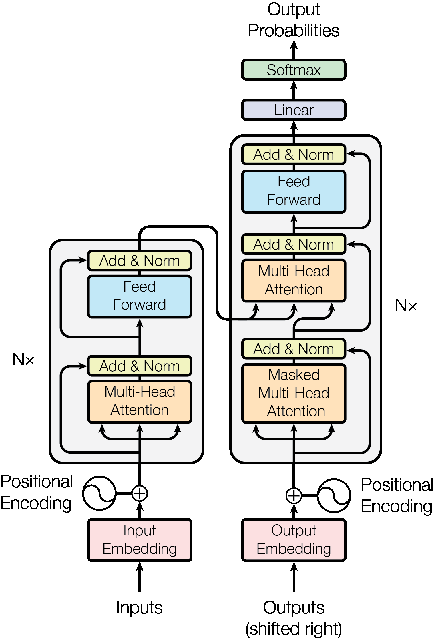
Figure 3: The full Transformer architecture. Left: the encoder stack. Right: the decoder stack. Input tokens are embedded and combined with positional encodings, then processed through \(N = 6\) identical layers. Each encoder layer contains multi-head self-attention followed by a feed-forward network. Each decoder layer adds cross-attention between self-attention and FFN. Residual connections and layer normalization wrap every sub-layer.
The Encoder is a stack of \(N = 6\) identical layers. Each layer has two sub-layers:
Each sub-layer is wrapped with a residual connection and layer normalization. All sub-layers and embeddings produce outputs of dimension \(d_\text{model} = 512\).
The encoder processes the entire input in parallel. After 6 layers, each position’s representation has been enriched by attending to all other positions, with progressively more abstract features captured at higher layers.
The Decoder is also a stack of \(N = 6\) identical layers, but each layer has three sub-layers:
The masking in the first sub-layer is critical. During training, we know the full target sentence, but we must prevent the model from “cheating” by looking at future words. The mask sets attention scores for future positions to \(-\infty\), which softmax converts to weight 0. This preserves the auto-regressive property: the prediction for position \(i\) depends only on positions 1 through \(i-1\).
Three uses of attention. The Transformer uses multi-head attention in three distinct configurations:
| Attention Type | Queries From | Keys/Values From | Masking |
|---|---|---|---|
| Encoder self-attention | Encoder layer \(l-1\) | Encoder layer \(l-1\) | None |
| Decoder self-attention | Decoder layer \(l-1\) | Decoder layer \(l-1\) | Future positions masked |
| Cross-attention | Decoder layer \(l-1\) | Encoder output | None |
Training. The model is trained on pairs of sentences (e.g., English-French). The input goes through the encoder. The target sentence (shifted right by one position, so the model predicts each word from all previous words) goes through the decoder. The model outputs a probability distribution over the vocabulary for each position, and the loss is the cross-entropy (a measure of how far the predicted probability distribution is from the true answer: \(-\log P(\text{correct word})\)) between these predictions and the actual next words.
The paper uses a custom learning rate schedule:
\[lrate = d_\text{model}^{-0.5} \cdot \min(step\_num^{-0.5}, \; step\_num \cdot warmup\_steps^{-1.5})\]
The learning rate increases linearly for 4000 steps (warmup), then decays proportionally to \(1 / \sqrt{step}\). The warmup is necessary because the Adam optimizer’s second-moment estimates are inaccurate at the start of training – large learning rates would cause unstable updates.
Inference (generation). Unlike training, inference is sequential: the decoder generates one token at a time. At each step, it feeds all previously generated tokens through the decoder, attends to the encoder output, and predicts the next token. This auto-regressive process continues until a stop token is produced.
Results. On English-to-German translation, the Transformer (big) achieved 28.4 BLEU (a standard metric for translation quality that measures overlap of word sequences between the model’s output and reference translations), beating all previous models including ensembles (multiple models combined) by over 2 points. The base model trained in just 12 hours on 8 GPUs at a cost of \(3.3 \times 10^{18}\) FLOPs (floating-point operations, a measure of total computation) – 3-60x cheaper than competing approaches. The architecture also generalized to English constituency parsing (analyzing the grammatical structure of sentences into nested phrases) without task-specific modifications.
Let’s trace a mini translation example through a simplified Transformer.
Input: “I eat” (English, 2 tokens) Target: “Je mange” (French, 2 tokens)
Step 1: Input embedding + positional encoding.
Token embeddings (dimension \(d_\text{model} = 4\) for this example):
Add positional encodings (from Lesson 5):
Encoder input:
Step 2: Encoder (1 layer for simplicity).
Self-attention: “I” and “eat” attend to each other. Suppose after attention:
FFN + residual + LayerNorm produces the final encoder output, call it \(\text{enc}\).
Step 3: Decoder generates “Je” (position 0).
Decoder input: start token embedding + position 0 encoding.
Step 4: Decoder generates “mange” (position 1).
Decoder input: [start token, “Je”] + position encodings.
The model is trained so that at every position, the predicted token matches the target. Once trained, the encoder processes the entire English sentence in parallel, and the decoder generates French tokens one at a time.
Recall: The Transformer decoder has three sub-layers. Name them in order and explain what each one does. Which one connects the encoder and decoder?
Apply: The base Transformer has \(N = 6\) layers, \(d_\text{model} = 512\), \(d_{ff} = 2048\), \(h = 8\) attention heads. Count the parameters in a single encoder layer: (a) multi-head self-attention has 4 projection matrices \(W^Q\), \(W^K\), \(W^V\) (each \(512 \times 64\), times 8 heads) and \(W^O\) (\(512 \times 512\)); (b) the FFN has \(W_1\) (\(512 \times 2048\)) and \(W_2\) (\(2048 \times 512\)). Sum them up. Then multiply by 6 layers for the full encoder.
Extend: During training, the entire target sequence is processed in parallel (the mask just prevents cheating). During inference, the decoder generates one token at a time. Why can’t inference be parallelized the same way as training? What fundamental property of auto-regressive generation prevents this?
Explain why the Transformer eliminates the sequential bottleneck of RNNs. What is the maximum path length between any two positions in a Transformer vs. an RNN, and why does this matter for learning long-range dependencies?
Why does the Transformer use scaling by \(\sqrt{d_k}\) in its attention mechanism? Walk through what would happen without scaling when \(d_k = 64\), including the effect on softmax gradients.
Compare the encoder-decoder structure of the Transformer to the encoder-decoder in the VAE (see Auto-Encoding Variational Bayes). Both have an encoder that produces a representation and a decoder that generates output from it. What are the key differences in what these encoders and decoders do?
The Transformer has \(O(n^2)\) memory and compute complexity in sequence length \(n\). For a 512-token sequence with \(d_\text{model} = 512\), how many entries does the attention weight matrix have? What about a 100,000-token document? Why does this quadratic scaling limit the Transformer’s applicability?
The paper demonstrated results only on machine translation and constituency parsing. Given what you know about how the Transformer works (self-attention, positional encoding, encoder-decoder), what properties make it potentially useful for other tasks like text classification, question answering, or image processing? What would need to change for each task?
Implement a single-layer Transformer encoder in numpy that processes a toy 3-word sentence through self-attention, a feed-forward network, and residual connections – producing context-aware representations for each word.
import numpy as np

np.random.seed(42)

# ── Hyperparameters ──────────────────────────────────────────────
SEQ_LEN = 3        # number of tokens
D_MODEL = 8        # embedding / model dimension
D_FF = 32          # feed-forward hidden dimension
D_K = D_MODEL      # query/key dimension (single head)
D_V = D_MODEL      # value dimension (single head)

# ── Positional encoding ─────────────────────────────────────────
def positional_encoding(seq_len, d_model):
    """
    Compute sinusoidal positional encodings.
    Returns: array of shape (seq_len, d_model)
    """
    # TODO: Implement the positional encoding from the paper
    # For each position pos and each dimension i:
    #   PE(pos, 2i)   = sin(pos / 10000^(2i/d_model))
    #   PE(pos, 2i+1) = cos(pos / 10000^(2i/d_model))
    pass


# ── Softmax ──────────────────────────────────────────────────────
def softmax(x):
    """Row-wise softmax. x has shape (seq_len, seq_len)."""
    # TODO: Implement numerically stable softmax (subtract max per row)
    pass


# ── Layer normalization ──────────────────────────────────────────
def layer_norm(x, gamma, beta, eps=1e-5):
    """
    Apply layer normalization to each row of x.
    x: shape (seq_len, d_model)
    gamma: scale parameter, shape (d_model,)
    beta: shift parameter, shape (d_model,)
    Returns: normalized x with same shape
    """
    # TODO: Normalize each row to mean=0, var=1, then scale and shift
    pass


# ── Weight initialization ───────────────────────────────────────
def init_weights(fan_in, fan_out):
    """Xavier/Glorot initialization."""
    scale = np.sqrt(2.0 / (fan_in + fan_out))
    return np.random.randn(fan_in, fan_out) * scale


# ── Token embeddings (random for this toy example) ──────────────
# Three tokens: "the" (0), "cat" (1), "sat" (2)
embeddings = np.random.randn(SEQ_LEN, D_MODEL) * 0.5

print("Token embeddings (before positional encoding):")
print(f"  'the': {embeddings[0].round(3).tolist()}")
print(f"  'cat': {embeddings[1].round(3).tolist()}")
print(f"  'sat': {embeddings[2].round(3).tolist()}")

# ── Add positional encoding ─────────────────────────────────────
pe = positional_encoding(SEQ_LEN, D_MODEL)
x = embeddings + pe

print("\nAfter adding positional encoding:")
for i, token in enumerate(["the", "cat", "sat"]):
    print(f"  '{token}': {x[i].round(3).tolist()}")

# ── Self-Attention weights ───────────────────────────────────────
W_Q = init_weights(D_MODEL, D_K)    # query projection
W_K = init_weights(D_MODEL, D_K)    # key projection
W_V = init_weights(D_MODEL, D_V)    # value projection

# ── Attention layer norm parameters ──────────────────────────────
attn_gamma = np.ones(D_MODEL)
attn_beta = np.zeros(D_MODEL)

# ── FFN weights ──────────────────────────────────────────────────
W1 = init_weights(D_MODEL, D_FF)    # expand: d_model -> d_ff
b1 = np.zeros(D_FF)
W2 = init_weights(D_FF, D_MODEL)    # compress: d_ff -> d_model
b2 = np.zeros(D_MODEL)

# ── FFN layer norm parameters ────────────────────────────────────
ffn_gamma = np.ones(D_MODEL)
ffn_beta = np.zeros(D_MODEL)


# ── Forward pass ─────────────────────────────────────────────────

# Step 1: Scaled Dot-Product Attention
# TODO: Compute Q, K, V by projecting x through W_Q, W_K, W_V
# TODO: Compute scores = Q @ K^T / sqrt(D_K)
# TODO: Compute attention weights = softmax(scores)
# TODO: Compute attention output = weights @ V
# TODO: Residual connection + layer norm

print("\n── Self-Attention ──────────────────────────────────────")
# print attention weights matrix
# print output after residual + layer norm

# Step 2: Position-wise Feed-Forward Network
# TODO: hidden = ReLU(x @ W1 + b1)
# TODO: output = hidden @ W2 + b2
# TODO: Residual connection + layer norm

print("\n── Feed-Forward Network ────────────────────────────────")
# print number of active ReLU units
# print output after residual + layer norm

# ── Final output ─────────────────────────────────────────────────
print("\n── Final Encoder Output ────────────────────────────────")
# for i, token in enumerate(["the", "cat", "sat"]):
#     print(f"  '{token}': {output[i].round(3).tolist()}")

# ── Verify properties ────────────────────────────────────────────
print("\n── Verification ───────────────────────────────────────")
# Each output should have mean ≈ 0, var ≈ 1 (due to layer norm)
# for i, token in enumerate(["the", "cat", "sat"]):
#     print(f"  '{token}': mean={output[i].mean():.4f}, "
# f"var={output[i].var():.4f}")After implementing all TODOs, you should see output similar to:
Token embeddings (before positional encoding):
  'the': [0.248, -0.069, 0.323, ...]
  'cat': [-0.117, -0.234, 0.116, ...]
  'sat': [0.28, 0.567, -0.088, ...]

After adding positional encoding:
  'the': [0.248, 0.931, 0.323, ...]
  'cat': [0.724, 0.306, 0.126, ...]
  'sat': [1.189, -0.087, -0.078, ...]

── Self-Attention ──────────────────────────────────────
Attention weights:
  'the' attends to: the=0.38  cat=0.29  sat=0.33
  'cat' attends to: the=0.31  cat=0.41  sat=0.28
  'sat' attends to: the=0.35  cat=0.27  sat=0.38

── Feed-Forward Network ────────────────────────────────
Active ReLU units: 18 / 32

── Final Encoder Output ────────────────────────────────
  'the': [-0.632, 1.241, -0.419, 0.873, -1.102, 0.547, -0.213, -0.295]
  'cat': [0.419, -0.736, 1.087, -0.514, 0.168, -1.341, 0.623, 0.294]
  'sat': [-0.287, 0.893, -1.156, 0.412, 0.741, -0.102, 0.338, -0.839]

── Verification ───────────────────────────────────────
  'the': mean=0.0000, var=0.9999
  'cat': mean=-0.0000, var=0.9999
  'sat': mean=0.0000, var=0.9999
Key things to verify:
Note: exact numbers will vary due to random weight initialization.