An Image is Worth 16x16 Words: Course

Learning Objectives

By the end of this course, you will be able to:

1. Explain how a digital image is represented as a 3D array of numbers and why feeding raw pixels to a Transformer is impractical
2. Describe how ViT converts a 2D image into a 1D sequence of patch embeddings that a standard Transformer can process
3. Compute the patch embedding and position encoding step by hand for a small example image
4. Trace an input through the full ViT forward pass: patching, embedding, Transformer encoder layers, and classification output
5. Explain inductive bias and why ViT needs more training data than convolutional neural networks (CNNs) to achieve the same performance
6. Evaluate the tradeoff between built-in architectural assumptions and learning from data at scale

Prerequisites

• Matrix multiplication and linear projections – multiplying a vector by a matrix to transform it between spaces. Basic linear algebra is sufficient.
• The softmax function – converts a vector of real numbers into a probability distribution. Used in the Transformer’s attention mechanism.
• The Transformer architecture – self-attention, multi-head attention, encoder structure, residual connections (see Attention Is All You Need)
• BERT’s [CLS] token – the concept of a special classification token prepended to an input sequence (see BERT)
• Transfer learning – pre-training on a large dataset then fine-tuning on a smaller target task (see Improving Language Understanding by Generative Pre-Training)

Lesson 1: Images as Numbers

Before we can apply any model to images, we need to understand how a computer represents an image. This lesson covers the data format that ViT takes as input.

Explanation

A digital photograph is a grid of tiny colored squares called pixels (short for “picture elements”). Each pixel’s color is described by three numbers – one for how much red, one for green, one for blue. These values typically range from 0 to 255, where 0 means none of that color and 255 means maximum intensity. Mixing these three channels produces any color: [255, 0, 0] is pure red, [0, 0, 0] is black, [255, 255, 255] is white.

A computer stores an image as a 3-dimensional array (a tensor) of shape \(H \times W \times C\), where:

• \(H\) is the height in pixels
• \(W\) is the width in pixels
• \(C\) is the number of color channels (3 for RGB)

A 224x224 RGB image – the standard input size for many image classifiers – is a tensor of shape \(224 \times 224 \times 3\), containing \(224 \times 224 \times 3 = 150{,}528\) individual numbers.

Why does this matter for Transformers? The Transformer architecture (see Attention Is All You Need) processes a sequence of tokens using self-attention, where every token attends to every other token. Self-attention computes a score between every pair of tokens, so its cost scales with the square of the sequence length: \(O(N^2)\). If we treated every pixel as a token, a 224x224 image would be a sequence of \(224 \times 224 = 50{,}176\) tokens. The attention matrix alone would have \(50{,}176^2 \approx 2.5\) billion entries – far too expensive for practical use. We need a way to reduce this sequence length dramatically.

Worked Example

Consider a tiny 4x4 RGB image. It has shape \(4 \times 4 \times 3\) and contains \(4 \times 4 \times 3 = 48\) numbers. Here is what it looks like as an array (showing just the red channel for brevity):

Red channel:         Green channel:       Blue channel:
[[120, 130, 200, 210],  [[100, 110, 50, 55],   [[ 80,  85, 30, 35],
 [125, 135, 205, 215],   [105, 115, 55, 60],    [ 82,  88, 32, 38],
 [ 40,  45,  50,  55],   [150, 155, 160, 165],  [120, 125, 130, 135],
 [ 42,  48,  52,  58]]   [152, 158, 162, 168]]  [122, 128, 132, 138]]

The pixel at position (0, 0) – top-left corner – has RGB values [120, 100, 80], a brownish color. The pixel at (0, 2) has values [200, 50, 30], a reddish color.

If we treated each pixel as a separate token, this tiny image would produce a sequence of \(4 \times 4 = 16\) tokens. The attention matrix would be \(16 \times 16 = 256\) entries. For a real 224x224 image, the same approach would require a \(50{,}176 \times 50{,}176\) attention matrix – roughly 10,000 times larger than what fits in memory.

Exercises

Recall: What are the three color channels in an RGB image, and what does each one represent?

Apply: A 320x256 RGB image has shape \(320 \times 256 \times 3\). How many total numbers does it contain? If each pixel were treated as a Transformer token, how many entries would the self-attention matrix have?

Extend: In practice, pixel values (0-255) are normalized to the range [0, 1] or [-1, 1] before feeding them to a neural network. Why might large integer values (like 200) cause problems during training? (Hint: think about what happens when you multiply large numbers together repeatedly.)

Lesson 2: From Pixels to Patches

Treating every pixel as a separate token is too expensive. This lesson introduces the key idea that makes ViT practical: chopping the image into patches and treating each patch as a single token.

Explanation

Think of how you might describe a photograph to someone over the phone. You would not say “pixel 1 is brown, pixel 2 is slightly lighter brown, pixel 3 is…” – you would say “there’s a dog in the lower-left corner, green grass underneath, blue sky at the top.” You naturally group the image into meaningful chunks.

ViT does something similar, though in a cruder way: it divides the image into a fixed grid of non-overlapping square patches, each \(P \times P\) pixels. For example, with patch size \(P = 16\), a 224x224 image becomes a grid of \(14 \times 14 = 196\) patches. Each patch captures a small region of the image – roughly the size of a thumbnail.

The number of patches \(N\) is:

\[N = \frac{H \times W}{P^2}\]

where \(H\) and \(W\) are the image height and width, and \(P\) is the patch size.

• \(N\) is the number of patches (and the sequence length for the Transformer)
• \(H \times W\) is the total number of pixels
• \(P^2\) is the number of pixels per patch

This reduces the sequence length from 50,176 pixels to just 196 patches – a 256x reduction. The attention matrix shrinks from 2.5 billion entries to \(196^2 = 38{,}416\) entries, which is entirely manageable.

Each patch is then flattened into a single vector. A \(P \times P\) patch from an RGB image has \(P \times P \times C\) values (width times height times color channels). For \(P = 16\) and \(C = 3\), each flattened patch is a vector of length \(16 \times 16 \times 3 = 768\).

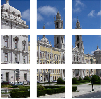
Figure 1: ViT’s patching process. An image is divided into a 3x3 grid of non-overlapping patches (left), and these patches are rearranged into a linear sequence (right). In practice, a 224x224 image with 16x16 patches yields 196 patches, not 9.

The grid order is row by row, left to right, top to bottom – the same reading order as English text. Patch 1 is the top-left corner, patch 2 is one step to the right, and so on.

Worked Example

Take our 4x4 RGB image from Lesson 1 and use patch size \(P = 2\). The number of patches is:

\[N = \frac{4 \times 4}{2^2} = \frac{16}{4} = 4\]

The image is divided into a 2x2 grid of patches, each 2x2 pixels. Each flattened patch is a vector of length \(2 \times 2 \times 3 = 12\).

Patch 1 (top-left, rows 0-1, columns 0-1):

Red:   [[120, 130], [125, 135]]
Green: [[100, 110], [105, 115]]
Blue:  [[ 80,  85], [ 82,  88]]

Flattened (interleaving channels per pixel): \(x_p^1 = [120, 100, 80, 130, 110, 85, 125, 105, 82, 135, 115, 88]\)

Patch 2 (top-right, rows 0-1, columns 2-3):

Red:   [[200, 210], [205, 215]]
Green: [[ 50,  55], [ 55,  60]]
Blue:  [[ 30,  35], [ 32,  38]]

Flattened: \(x_p^2 = [200, 50, 30, 210, 55, 35, 205, 55, 32, 215, 60, 38]\)

Patch 3 (bottom-left) and Patch 4 (bottom-right) follow the same pattern. We now have 4 vectors of length 12 instead of 16 individual pixels – a 4x reduction in sequence length.

Exercises

Recall: Why does ViT use patches instead of individual pixels as tokens?

Apply: An image has dimensions \(384 \times 384 \times 3\) (RGB). Using patch size \(P = 16\), how many patches \(N\) does this produce? What is the length of each flattened patch vector?

Extend: The paper uses the notation “ViT-L/16” where 16 is the patch size. ViT-L/32 uses 32x32 patches instead. How does doubling the patch size affect (a) the number of patches, (b) the length of each flattened patch vector, and (c) the computational cost of self-attention? What information might be lost by using larger patches?

Lesson 3: Patch Embeddings and Position Encoding

Flattened patches are raw pixel values – they are not yet in a form useful for a Transformer. This lesson covers how ViT projects patches into an embedding space and adds position information, following the same pattern used for word embeddings in NLP Transformers.

Explanation

In NLP, each word is converted to a dense vector (an embedding) before being fed to a Transformer. The word “cat” might become a 768-dimensional vector where each dimension captures some aspect of meaning. ViT does the same thing for image patches: each flattened patch is multiplied by a learned matrix to produce a patch embedding.

The embedding equation from the paper is:

\[\mathbf{z}_0 = [\mathbf{x}_\text{class};\; \mathbf{x}_p^1 \mathbf{E};\; \mathbf{x}_p^2 \mathbf{E};\; \cdots;\; \mathbf{x}_p^N \mathbf{E}] + \mathbf{E}_{pos}\]

where \(\mathbf{E} \in \mathbb{R}^{(P^2 \cdot C) \times D}\) and \(\mathbf{E}_{pos} \in \mathbb{R}^{(N+1) \times D}\).

• \(\mathbf{x}_p^i\) is the \(i\)-th flattened patch, a vector of length \(P^2 \cdot C\)
• \(\mathbf{E}\) is the patch embedding matrix that projects each patch vector from \(P^2 \cdot C\) dimensions to \(D\) dimensions (the Transformer’s hidden size)
• \(\mathbf{x}_\text{class}\) is a learnable class token, a single \(D\)-dimensional vector prepended to the sequence
• \(\mathbf{E}_{pos}\) is the position embedding matrix: \(N + 1\) vectors (one per patch plus one for the class token), each \(D\)-dimensional
• \(\mathbf{z}_0\) is the resulting \((N+1) \times D\) matrix fed into the first Transformer layer

This equation does three things at once:

First, each patch is projected into embedding space. The multiplication \(\mathbf{x}_p^i \mathbf{E}\) takes a raw patch vector (pixel values) and transforms it into a learned representation. For ViT-Base, both the input and output are 768-dimensional (\(P^2 \cdot C = 16^2 \cdot 3 = 768\) and \(D = 768\)), but the projection matrix \(\mathbf{E}\) learns to map from “pixel space” to “feature space.”

Second, a class token \(\mathbf{x}_\text{class}\) is prepended. This is borrowed from BERT (see BERT): a learnable vector that starts blank and accumulates information about the whole image as it passes through the Transformer layers. At the end, this single vector is used to classify the image.

Third, position embeddings \(\mathbf{E}_{pos}\) are added. Without position information, the Transformer would treat the patches as a bag – it would not know that patch 1 is in the top-left and patch 196 is in the bottom-right. The position embeddings are learned vectors (one per position) that encode where each patch came from. They are added element-wise to the patch embeddings.

A striking finding: even though the position embeddings are 1D (just numbered 1 through \(N\), with no 2D grid information), the model learns 2D spatial structure on its own. Nearby patches end up with similar position embeddings, and row-column patterns emerge automatically.

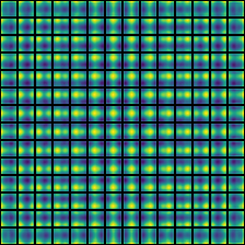
Figure 2: Cosine similarity between position embeddings for ViT-L/16 (14x14 grid = 196 patches). Each small grid shows one patch’s similarity to all others. The bright spots near each cell’s center show that nearby patches have similar embeddings. Row and column structure is clearly visible – the model discovers 2D spatial relationships from 1D position indices alone.

Worked Example

Let us trace through the embedding step with concrete numbers. Suppose we have a tiny image that produces \(N = 4\) patches, each of length \(P^2 \cdot C = 12\) (from our 4x4 image with \(P = 2\)). We use embedding dimension \(D = 3\) (tiny, for illustration).

Our four flattened patches (using normalized values in [0, 1]):

• \(\mathbf{x}_p^1 = [0.47, 0.39, 0.31, 0.51, 0.43, 0.33, 0.49, 0.41, 0.32, 0.53, 0.45, 0.35]\)
• \(\mathbf{x}_p^2 = [0.78, 0.20, 0.12, 0.82, 0.22, 0.14, 0.80, 0.22, 0.13, 0.84, 0.24, 0.15]\)
• \(\mathbf{x}_p^3 = [0.16, 0.59, 0.47, 0.18, 0.61, 0.49, 0.16, 0.59, 0.47, 0.18, 0.61, 0.49]\)
• \(\mathbf{x}_p^4 = [0.20, 0.63, 0.51, 0.22, 0.65, 0.53, 0.20, 0.63, 0.51, 0.22, 0.65, 0.53]\)

The embedding matrix \(\mathbf{E}\) has shape \(12 \times 3\). Suppose after the multiplication \(\mathbf{x}_p^i \mathbf{E}\), we get:

The class token starts as a learned vector, say \(\mathbf{x}_\text{class} = [0.01, 0.01, 0.01]\).

We prepend it to get a \(5 \times 3\) matrix (5 tokens: 1 class + 4 patches):

\[[\mathbf{x}_\text{class};\; \mathbf{x}_p^1 \mathbf{E};\; \mathbf{x}_p^2 \mathbf{E};\; \mathbf{x}_p^3 \mathbf{E};\; \mathbf{x}_p^4 \mathbf{E}] = \begin{bmatrix} 0.01 & 0.01 & 0.01 \\ 0.42 & -0.15 & 0.73 \\ 0.91 & 0.33 & -0.20 \\ -0.28 & 0.67 & 0.51 \\ -0.12 & 0.78 & 0.39 \end{bmatrix}\]

Now add position embeddings \(\mathbf{E}_{pos}\), a \(5 \times 3\) matrix (one row per position):

\[\mathbf{E}_{pos} = \begin{bmatrix} 0.10 & -0.05 & 0.02 \\ 0.08 & 0.03 & -0.01 \\ -0.04 & 0.07 & 0.05 \\ 0.03 & -0.02 & 0.09 \\ -0.06 & 0.04 & 0.06 \end{bmatrix}\]

The final input to the Transformer is:

\[\mathbf{z}_0 = \begin{bmatrix} 0.11 & -0.04 & 0.03 \\ 0.50 & -0.12 & 0.72 \\ 0.87 & 0.40 & -0.15 \\ -0.25 & 0.65 & 0.60 \\ -0.18 & 0.82 & 0.45 \end{bmatrix}\]

This \(5 \times 3\) matrix is a sequence of 5 tokens, each with 3 features – ready for the Transformer encoder.

Exercises

Recall: What are the three components that are combined to form \(\mathbf{z}_0\) (the input to the first Transformer layer)?

Apply: For ViT-Base with a 224x224 RGB image and patch size \(P = 16\): what is the shape of the embedding matrix \(\mathbf{E}\)? What is the shape of the position embedding matrix \(\mathbf{E}_{pos}\)? What is the shape of \(\mathbf{z}_0\)?

Extend: The paper found that 1D position embeddings work just as well as 2D position embeddings. Why might this be the case for 14x14 patch grids, even though images are inherently 2D? (Hint: how many positions does the model need to learn representations for, and how does that compare to the embedding dimension?)

Lesson 4: Self-Attention Over Patches

With the image converted to a sequence of patch embeddings, the Transformer processes them using self-attention. This lesson reviews how self-attention works and what it means when applied to image patches instead of words.

Explanation

Self-attention (covered in detail in Attention Is All You Need) lets each token in a sequence look at every other token and decide how much information to gather from each. In NLP, this lets the word “it” attend to “the cat” earlier in the sentence to resolve what “it” refers to. For image patches, self-attention lets each patch gather information from all other patches – a patch showing a dog’s ear can attend to a patch showing the dog’s body to build a richer representation.

For a single attention head, the computation is:

\[[\mathbf{q}, \mathbf{k}, \mathbf{v}] = \mathbf{z} \mathbf{U}_{qkv}, \quad \mathbf{U}_{qkv} \in \mathbb{R}^{D \times 3D_h}\]

\[A = \operatorname{softmax}(\mathbf{q}\mathbf{k}^\top / \sqrt{D_h}), \quad A \in \mathbb{R}^{N \times N}\]

\[\operatorname{SA}(\mathbf{z}) = A\mathbf{v}\]

• \(\mathbf{z}\) is the input sequence: \(N\) tokens (patches + class token), each of dimension \(D\)
• \(\mathbf{U}_{qkv}\) is a learned projection matrix that produces three vectors per token: a query \(\mathbf{q}\), a key \(\mathbf{k}\), and a value \(\mathbf{v}\), each of dimension \(D_h\)
• \(\mathbf{q}\mathbf{k}^\top\) computes the dot product between every pair of query and key vectors, producing an \(N \times N\) matrix of raw similarity scores
• Dividing by \(\sqrt{D_h}\) prevents scores from becoming too large, which would push softmax into regions where gradients vanish
• \(\operatorname{softmax}\) converts each row into a probability distribution (non-negative values summing to 1)
• \(A\mathbf{v}\) produces a weighted combination of value vectors: each token’s new representation is a mix of all tokens’ values, weighted by relevance

For multi-head self-attention (MSA) with \(k\) heads, the model runs \(k\) independent attention operations in parallel, each with \(D_h = D/k\) dimensions, and concatenates the results:

\[\operatorname{MSA}(\mathbf{z}) = [\operatorname{SA}_1(\mathbf{z});\; \operatorname{SA}_2(\mathbf{z});\; \cdots;\; \operatorname{SA}_k(\mathbf{z})] \, \mathbf{U}_{msa}, \quad \mathbf{U}_{msa} \in \mathbb{R}^{k \cdot D_h \times D}\]

• Each head \(\operatorname{SA}_i\) operates on \(D_h = D/k\) dimensions
• The \(k\) outputs are concatenated to form a \(k \cdot D_h = D\) dimensional vector
• \(\mathbf{U}_{msa}\) is a final projection matrix that mixes information across heads

Multiple heads let the model attend to different types of relationships simultaneously. In ViT, the paper found that different heads specialize: some attend locally (nearby patches), others attend globally (across the entire image), and this varies by layer depth. Early layers have a mix of local and global heads; later layers attend almost entirely globally.

The critical difference from CNNs: a convolutional layer can only look at a small local neighborhood (e.g., 3x3 pixels). It takes many stacked layers before information from distant parts of the image can interact. Self-attention lets every patch attend to every other patch in a single layer – a patch in the top-left corner can directly interact with a patch in the bottom-right corner from the very first layer.

Worked Example

Let us compute single-head self-attention for 3 tokens (1 class token + 2 patches) with \(D = 4\) and \(D_h = 4\).

Input \(\mathbf{z}\) (after embedding and position encoding):

\[\mathbf{z} = \begin{bmatrix} 0.11 & -0.04 & 0.03 & 0.20 \\ 0.50 & -0.12 & 0.72 & 0.15 \\ 0.87 & 0.40 & -0.15 & 0.30 \end{bmatrix}\]

Suppose after the \(\mathbf{U}_{qkv}\) projection, we get:

\[ \mathbf{q} = \begin{bmatrix} 0.1 & 0.2 & -0.1 & 0.3 \\ 0.4 & -0.3 & 0.5 & 0.1 \\ 0.2 & 0.6 & 0.1 & -0.2 \end{bmatrix}, \quad \mathbf{k} = \begin{bmatrix} 0.3 & 0.1 & 0.2 & -0.1 \\ -0.2 & 0.4 & 0.1 & 0.3 \\ 0.5 & -0.1 & 0.3 & 0.2 \end{bmatrix} \]

Step 1: compute \(\mathbf{q}\mathbf{k}^\top\) (3x3 matrix):

Row 0 of \(\mathbf{q}\) dotted with each row of \(\mathbf{k}\):

• \((0.1)(0.3) + (0.2)(0.1) + (-0.1)(0.2) + (0.3)(-0.1) = 0.03 + 0.02 - 0.02 - 0.03 = 0.00\)
• \((0.1)(-0.2) + (0.2)(0.4) + (-0.1)(0.1) + (0.3)(0.3) = -0.02 + 0.08 - 0.01 + 0.09 = 0.14\)
• \((0.1)(0.5) + (0.2)(-0.1) + (-0.1)(0.3) + (0.3)(0.2) = 0.05 - 0.02 - 0.03 + 0.06 = 0.06\)

\[\mathbf{q}\mathbf{k}^\top = \begin{bmatrix} 0.00 & 0.14 & 0.06 \\ 0.27 & -0.14 & 0.30 \\ 0.11 & 0.26 & 0.06 \end{bmatrix}\]

Step 2: scale by \(1/\sqrt{D_h} = 1/\sqrt{4} = 0.5\):

\[\text{scaled} = \begin{bmatrix} 0.00 & 0.07 & 0.03 \\ 0.14 & -0.07 & 0.15 \\ 0.06 & 0.13 & 0.03 \end{bmatrix}\]

Step 3: apply softmax to each row:

Row 0: \(\operatorname{softmax}([0.00, 0.07, 0.03]) = [0.327, 0.351, 0.337]\) (roughly uniform – the class token attends to both patches similarly)

The attention weights tell us how much each token “looks at” each other token. The class token (row 0) attends roughly equally to both patches. In a real ViT with 196 patches, this attention pattern would reveal which parts of the image the model considers most important.

Exercises

Recall: What three vectors does self-attention compute for each token, and what role does each play?

Apply: In ViT-Base, \(D = 768\) and there are \(k = 12\) attention heads. What is \(D_h\) for each head? With \(N = 197\) tokens (196 patches + 1 class token), what is the shape of the attention matrix \(A\) for a single head?

Extend: A CNN’s first layer typically uses 3x3 filters, so each output pixel depends only on a 3x3 neighborhood. How many convolutional layers would you need to stack before a pixel in the top-left can be influenced by a pixel in the bottom-right of a 224x224 image? Compare this to how many Transformer layers are needed for the same interaction.

Lesson 5: The Transformer Encoder Block

Each Transformer layer applies self-attention followed by a feed-forward network, with layer normalization and residual connections wrapping each sub-block. This lesson covers how these components fit together in ViT.

Explanation

A single Transformer encoder layer in ViT has two sub-blocks stacked on top of each other. The first sub-block applies multi-head self-attention:

\[\mathbf{z}'_\ell = \operatorname{MSA}(\operatorname{LN}(\mathbf{z}_{\ell-1})) + \mathbf{z}_{\ell-1}, \quad \ell = 1 \ldots L\]

• \(\mathbf{z}_{\ell-1}\) is the output from the previous layer (or \(\mathbf{z}_0\) for the first layer)
• \(\operatorname{LN}\) is layer normalization: it normalizes each vector to have zero mean and unit variance, stabilizing training. Think of it as “resetting the scale” of each vector before processing.
• \(\operatorname{MSA}\) is multi-head self-attention (from Lesson 4)
• \(+ \mathbf{z}_{\ell-1}\) is a residual connection (shortcut): the original input is added back to the output. This helps training in two ways – it gives gradients a direct path backward through the network, and it lets each layer learn a small refinement on top of what came before rather than having to reconstruct the entire representation from scratch.
• \(\mathbf{z}'_\ell\) is the intermediate output after this sub-block

The second sub-block applies a feed-forward network (called an MLP):

\[\mathbf{z}_\ell = \operatorname{MLP}(\operatorname{LN}(\mathbf{z}'_\ell)) + \mathbf{z}'_\ell, \quad \ell = 1 \ldots L\]

• \(\operatorname{MLP}\) is a two-layer feed-forward network: the first layer expands the dimension (by 4x in ViT, e.g., from 768 to 3072), applies GELU activation (a smooth non-linear function), and the second layer projects back down to \(D\)
• The same residual-connection-around-layer-norm pattern is used
• \(\mathbf{z}_\ell\) is the final output of this layer

Notice the order: LayerNorm comes before the operation (attention or MLP), not after. This is called “pre-norm” and differs from the original Transformer which applied LayerNorm after. Pre-norm tends to be more stable during training.

The attention sub-block mixes information across tokens (patches). The MLP sub-block processes each token independently – it transforms each token’s representation without looking at other tokens. Together, they form a pattern: mix information (attention) then process individually (MLP), repeated \(L\) times.

Worked Example

Let us trace through one encoder layer with 3 tokens (\(N = 3\)) and \(D = 4\).

Input \(\mathbf{z}_0\):

\[\mathbf{z}_0 = \begin{bmatrix} 0.11 & -0.04 & 0.03 & 0.20 \\ 0.50 & -0.12 & 0.72 & 0.15 \\ 0.87 & 0.40 & -0.15 & 0.30 \end{bmatrix}\]

Step 1: LayerNorm on each row. For row 0, \(\text{mean} = (0.11 - 0.04 + 0.03 + 0.20)/4 = 0.075\), then subtract mean and divide by standard deviation. Suppose after LN:

\[\operatorname{LN}(\mathbf{z}_0) = \begin{bmatrix} 0.21 & -0.70 & -0.27 & 0.76 \\ 0.33 & -0.78 & 1.05 & -0.60 \\ 0.92 & 0.17 & -1.28 & 0.19 \end{bmatrix}\]

Step 2: MSA on the normalized input. Suppose the attention output is:

\[\operatorname{MSA}(\operatorname{LN}(\mathbf{z}_0)) = \begin{bmatrix} 0.05 & -0.10 & 0.08 & 0.02 \\ 0.12 & 0.06 & -0.03 & 0.09 \\ -0.04 & 0.15 & 0.07 & -0.08 \end{bmatrix}\]

Step 3: Residual connection – add back \(\mathbf{z}_0\):

\[\mathbf{z}'_1 = \begin{bmatrix} 0.16 & -0.14 & 0.11 & 0.22 \\ 0.62 & -0.06 & 0.69 & 0.24 \\ 0.83 & 0.55 & -0.08 & 0.22 \end{bmatrix}\]

Step 4: LayerNorm on \(\mathbf{z}'_1\), then MLP, then residual connection to get \(\mathbf{z}_1\).

The MLP expands each 4-dim vector to \(4 \times 4 = 16\) dimensions, applies GELU, then projects back to 4. Suppose the final output is:

\[\mathbf{z}_1 = \begin{bmatrix} 0.20 & -0.18 & 0.15 & 0.28 \\ 0.71 & -0.01 & 0.62 & 0.30 \\ 0.79 & 0.61 & -0.02 & 0.18 \end{bmatrix}\]

This \(\mathbf{z}_1\) is the input to layer 2. After \(L\) such layers, we extract the class token for classification.

Exercises

Recall: In what order are the four operations applied within a single ViT encoder layer? (List all four: LayerNorm, MSA, LayerNorm, MLP, and specify where the residual connections go.)

Apply: ViT-Base has \(D = 768\) and the MLP hidden dimension is 3072. How many parameters does the MLP block of a single layer have? (Hint: two linear layers – one expanding from 768 to 3072, one projecting from 3072 to 768. Count weights and biases.)

Extend: The residual connection adds the input directly to the output: \(\mathbf{z}'_\ell = f(\mathbf{z}_{\ell-1}) + \mathbf{z}_{\ell-1}\). This means the layer only needs to learn \(f(\mathbf{z}) = \mathbf{z}'_\ell - \mathbf{z}_{\ell-1}\), the difference from the input. Why is learning a small correction easier than learning the full transformation from scratch?

Lesson 6: The Complete Vision Transformer

This lesson assembles all the pieces into the full ViT architecture and covers how the model produces a classification output.

Explanation

The complete ViT forward pass has four stages, each captured by one equation from the paper:

Stage 1: Patch embedding (Lesson 3)

\[\mathbf{z}_0 = [\mathbf{x}_\text{class};\; \mathbf{x}_p^1 \mathbf{E};\; \mathbf{x}_p^2 \mathbf{E};\; \cdots;\; \mathbf{x}_p^N \mathbf{E}] + \mathbf{E}_{pos}\]

Split image into patches, project each into embedding space, prepend class token, add position embeddings.

Stage 2: Self-attention sub-block (Lesson 5), repeated \(L\) times

\[\mathbf{z}'_\ell = \operatorname{MSA}(\operatorname{LN}(\mathbf{z}_{\ell-1})) + \mathbf{z}_{\ell-1}, \quad \ell = 1 \ldots L\]

Stage 3: MLP sub-block (Lesson 5), repeated \(L\) times

\[\mathbf{z}_\ell = \operatorname{MLP}(\operatorname{LN}(\mathbf{z}'_\ell)) + \mathbf{z}'_\ell, \quad \ell = 1 \ldots L\]

Stage 4: Classification output

\[\mathbf{y} = \operatorname{LN}(\mathbf{z}_L^0)\]

• \(\mathbf{z}_L^0\) is the class token’s output vector after the final (\(L\)-th) Transformer layer (the superscript 0 means position 0 – the class token)
• \(\mathbf{y}\) is the normalized image representation
• This vector is fed to a classification head (a linear layer that maps from \(D\) dimensions to \(K\) classes)

The class token works like a “summary ticket” that travels through all \(L\) layers, gathering information from every patch through self-attention. By the final layer, it has seen the entire image and distilled it into a single vector.

The model comes in three sizes, mirroring BERT’s configurations:

Pre-training and fine-tuning. Like GPT (see Improving Language Understanding by Generative Pre-Training), ViT is first pre-trained on a large classification dataset (ImageNet-21k or JFT-300M), then fine-tuned on a smaller downstream task. During fine-tuning, the pre-trained classification head is replaced with a new zero-initialized linear layer sized for the target number of classes. Fine-tuning is often done at higher resolution (e.g., 384x384 instead of 224x224), which increases the number of patches. The pre-trained position embeddings are 2D-interpolated to handle the new grid size.

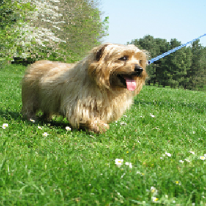
Figure 3: An input image shown to ViT-L/16. The model must classify this image.

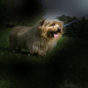
Figure 4: Attention rollout for the same image, computed by multiplying attention weights across all layers. Bright areas show where the model focuses. ViT learns to attend to the semantically relevant object (the dog) and suppress the background, without any built-in spatial assumptions.

Worked Example

Let us trace the full forward pass for a concrete (but tiny) example.

Input: a 4x4 RGB image, patch size \(P = 2\), embedding dimension \(D = 3\), \(L = 1\) layer, \(k = 1\) attention head.

Stage 1 (from Lesson 3): 4 patches, each flattened to length 12, projected to \(D = 3\), class token prepended, position embeddings added. Result: \(\mathbf{z}_0\) is a \(5 \times 3\) matrix (5 tokens).

Stages 2-3 (from Lesson 5): One encoder layer processes \(\mathbf{z}_0\):

• LayerNorm, MSA (each of the 5 tokens attends to all 5), residual connection \(\rightarrow \mathbf{z}'_1\)
• LayerNorm, MLP (each token processed independently), residual connection \(\rightarrow \mathbf{z}_1\)

Result: \(\mathbf{z}_1\) is still \(5 \times 3\).

Stage 4: Extract the class token (row 0 of \(\mathbf{z}_1\)), apply LayerNorm:

\[\mathbf{y} = \operatorname{LN}(\mathbf{z}_1^0) = \operatorname{LN}([0.20, -0.18, 0.28]) = [0.33, -1.31, 0.98]\]

Classification: multiply by a \(3 \times K\) weight matrix (the classification head). For \(K = 2\) classes (say, “dog” vs. “cat”):

\[\text{logits} = \mathbf{y} \cdot W_\text{head} = [0.33, -1.31, 0.98] \cdot \begin{bmatrix} 0.5 & -0.3 \\ -0.2 & 0.7 \\ 0.4 & 0.1 \end{bmatrix} = [0.82, -1.01]\]

Apply softmax: \(\operatorname{softmax}([0.82, -1.01]) = [0.86, 0.14]\). The model predicts class 0 (“dog”) with 86% confidence.

Exercises

Recall: After all Transformer layers are done, which specific vector from the output sequence does ViT use for classification, and why?

Apply: ViT-Large uses \(L = 24\) layers, \(D = 1024\), and 16 attention heads. For a 224x224 image with \(P = 16\) (so \(N = 196\) patches), how many tokens does the Transformer process? What is \(D_h\) per attention head?

Extend: During fine-tuning at 384x384 resolution (up from 224x224 at pre-training), the number of patches increases from 196 to \(384^2 / 16^2 = 576\). The pre-trained position embeddings have 197 entries (196 patches + 1 class token), but now we need 577. The paper uses 2D interpolation of the position embeddings to handle this. Why can’t we just add new randomly initialized position embeddings for the extra positions?

Lesson 7: Inductive Bias and the Power of Scale

This is the paper’s core finding: when you have enough data, a model with no built-in assumptions about images can match or beat models that were specifically designed for vision tasks. This lesson covers what inductive bias is, why ViT has less of it than CNNs, and why that turns out to be an advantage at scale.

Explanation

An inductive bias is a built-in assumption that a model makes about the structure of its input. Think of it like the difference between a custom-made tool and a general-purpose one. A corkscrew is designed specifically for opening wine bottles – it has a “built-in assumption” about the task. A pair of pliers is more general – it can grip anything, but it is worse at opening wine bottles specifically. If you only ever need to open wine bottles, the corkscrew wins. But if you encounter tasks that the corkscrew was not designed for, the pliers are more flexible.

CNNs are like the corkscrew. They have three strong inductive biases for vision:

1. Locality: convolutional filters look only at small neighborhoods (e.g., 3x3 pixels). This assumes that useful patterns are local.
2. Translation equivariance: the same filter is applied at every position. This assumes a pattern (like an edge) is equally useful regardless of where it appears.
3. Hierarchical structure: early layers detect simple features (edges), later layers combine them into complex features (eyes, faces). This assumes that visual features compose hierarchically.

ViT is like the pliers. It has almost no image-specific inductive biases:

• Self-attention is global from layer 1 – no locality assumption
• The MLP layers are the only local and translationally equivariant component
• The only place ViT uses 2D structure is when cutting the image into patches and when interpolating position embeddings during fine-tuning

The paper’s central experiment tests what happens when you train both architectures on datasets of increasing size:

With 1.3 million images, the CNN’s built-in assumptions about image structure give it an advantage – it does not need to learn from scratch that nearby pixels are related, because locality is baked in. But with 300 million images, ViT has enough data to discover these patterns on its own – and it discovers patterns that are more flexible than what the CNN’s fixed assumptions encode.

The results on ImageNet (after pre-training on JFT-300M):

ViT-L/16 matches the best CNN (BiT-L) at roughly 15x less compute. ViT-H/14 edges ahead of Noisy Student (the state-of-the-art CNN at the time) while using 5x less compute. The Transformer architecture is simply more efficient at converting compute into performance for vision tasks, once data is abundant.

This echoes a finding from the language domain. GPT (see Improving Language Understanding by Generative Pre-Training) showed that a general-purpose Transformer, pre-trained on enough text, beats task-specific architectures. The scaling laws paper (see Scaling Laws for Neural Language Models) showed that performance improves predictably with scale. ViT extends this pattern to vision: scale and data substitute for domain-specific architectural engineering.

The limitation is real though. Most organizations do not have 300 million labeled images. JFT-300M is a proprietary Google dataset. Until methods were developed to make ViT work with less data (DeiT, self-supervised pre-training with MAE/DINO), this was a significant practical constraint.

Worked Example

Let us quantify the inductive bias tradeoff with numbers from the paper.

On ImageNet-only pre-training (1.3M images):

• ViT-Base: 77.91% accuracy
• ViT-Large: 76.53% accuracy
• Difference: -1.38% (larger model is worse)

The larger ViT-Large has more parameters but no additional structural constraints. With only 1.3M images, it memorizes training data rather than learning generalizable features. This is classic overfitting: the model is too flexible for the amount of data.

On JFT-300M pre-training (303M images):

• ViT-Base: 84.15% accuracy
• ViT-Large: 87.12% accuracy
• Difference: +2.97% (larger model is better)

With 230x more data, the extra capacity of ViT-Large becomes an advantage rather than a liability. The model can now learn richer, more general features without overfitting.

Compare to ResNets on the same JFT-300M pre-training:

• ResNet152x2: 84.97% accuracy (563 exaFLOPs to pre-train)
• ViT-L/16: 87.12% accuracy (783 exaFLOPs)
• ViT-L/16 at 7 epochs: 86.30% (783 exaFLOPs)

ViT-L/16 beats ResNet152x2 by 2 percentage points with roughly comparable compute. The Transformer extracts more from the same data.

Exercises

Recall: Name three inductive biases that CNNs have for image processing that ViT does not.

Apply: A ViT-Base model pre-trained on ImageNet (1.3M images) achieves 77.91% accuracy. The same model pre-trained on JFT-300M (303M images) achieves 84.15%. What is the accuracy gain per 10x increase in dataset size? (Note: JFT is roughly 230x larger than ImageNet.)

Extend: The paper found that ViT needs roughly 14 million images before it starts matching CNNs. Self-supervised methods like MAE (Masked Autoencoders, 2022) later showed that ViT can match supervised performance without labels, by masking 75% of patches and training the model to reconstruct them. Why might self-supervised pre-training reduce ViT’s data requirement? (Hint: think about the relationship between the pretext task and the inductive biases that CNNs have built in.)

Comprehension Questions

1. ViT splits images into patches and treats them as tokens. What specific tradeoff does this create between computational cost and the granularity of visual information?

2. Why did the authors choose to use a [CLS] token for classification rather than averaging all patch embeddings? What is the practical difference, and what did the ablation study reveal?

3. ViT’s position embeddings are 1D (numbered sequentially), yet the model learns 2D spatial structure. What evidence from the paper demonstrates this, and what does it suggest about the Transformer’s ability to discover structure from data?

4. When ViT is pre-trained only on ImageNet (1.3M images), ViT-Large performs worse than ViT-Base. Explain why, and identify the minimum dataset size where larger models start to help.

5. How does ViT relate to GPT’s contribution? Both applied Transformers to domains previously dominated by specialized architectures. What is the common lesson, and where does the analogy break down?

Hands-On Project

Goal

Implement the ViT patch embedding and single-head self-attention forward pass from scratch in numpy, using a real (tiny) image.

Specification

• Input: a 4x4 RGB image (provided as a numpy array)
• Patch size: 2x2, yielding 4 patches
• Embedding dimension: 8
• One Transformer layer with single-head attention
• Output: the class token vector after one layer

Implement: (1) patch extraction and flattening, (2) linear projection to embedding space, (3) class token prepend and position embedding addition, (4) single-head self-attention, (5) MLP block, (6) extract class token output.

Starter Code

import numpy as np

np.random.seed(42)

# --- Input ---
# A 4x4 RGB image (values in [0, 1])
image = np.random.rand(4, 4, 3)
P = 2          # patch size
D = 8          # embedding dimension
N = (4 // P) * (4 // P)  # number of patches = 4
mlp_dim = 16   # MLP hidden dimension

# --- Step 1: Extract and flatten patches ---
def extract_patches(image, patch_size):
    """Split image into non-overlapping patches and flatten each.

    Args:
        image: numpy array of shape (H, W, C)
        patch_size: integer P, the side length of each square patch

    Returns:
        patches: numpy array of shape (N, P*P*C) where N = (H/P) * (W/P)
    """
    # TODO: Split the image into a grid of PxP patches.
    # Flatten each patch into a vector of length P*P*C.
    # Return them in row-major order (left to right, top to bottom).
    pass

patches = extract_patches(image, P)
assert patches.shape == (N, P * P * 3), f"Expected ({N}, {P*P*3}), got {patches.shape}"

# --- Step 2: Linear projection ---
E = np.random.randn(P * P * 3, D) * 0.02  # patch embedding matrix

def project_patches(patches, E):
    """Project flattened patches into embedding space.

    Args:
        patches: (N, P*P*C) array of flattened patches
        E: (P*P*C, D) projection matrix

    Returns:
        embeddings: (N, D) array
    """
    # TODO: Matrix multiply patches by E.
    pass

patch_embeddings = project_patches(patches, E)
assert patch_embeddings.shape == (N, D)

# --- Step 3: Prepend class token and add position embeddings ---
cls_token = np.random.randn(1, D) * 0.02  # learnable class token
E_pos = np.random.randn(N + 1, D) * 0.02  # position embeddings

def prepare_input(patch_embeddings, cls_token, E_pos):
    """Prepend class token and add position embeddings.

    Args:
        patch_embeddings: (N, D) array
        cls_token: (1, D) array
        E_pos: (N+1, D) position embeddings

    Returns:
        z0: (N+1, D) array -- the input to the Transformer
    """
    # TODO: Concatenate cls_token with patch_embeddings along axis 0,
    # then add position embeddings element-wise.
    pass

z0 = prepare_input(patch_embeddings, cls_token, E_pos)
assert z0.shape == (N + 1, D)

# --- Step 4: Layer Normalization ---
def layer_norm(x, eps=1e-6):
    """Apply layer normalization to each row of x.

    Args:
        x: (T, D) array where T is number of tokens

    Returns:
        normalized: (T, D) array where each row has mean ~0 and variance ~1
    """
    # TODO: For each row, subtract the mean and divide by the standard deviation.
    # Add eps to the denominator to avoid division by zero.
    pass

# --- Step 5: Single-head self-attention ---
W_qkv = np.random.randn(D, 3 * D) * 0.02  # combined QKV projection
W_out = np.random.randn(D, D) * 0.02       # output projection

def self_attention(z, W_qkv, W_out):
    """Compute single-head self-attention.

    Args:
        z: (T, D) input tokens
        W_qkv: (D, 3*D) combined projection for queries, keys, values
        W_out: (D, D) output projection

    Returns:
        output: (T, D) attention output
    """
    # TODO:
    # 1. Project z to get q, k, v by multiplying by W_qkv and splitting
    # 2. Compute attention scores: q @ k.T / sqrt(D)
    # 3. Apply softmax to each row of the scores
    # 4. Compute weighted sum: A @ v
    # 5. Project output through W_out
    pass

# --- Step 6: MLP block ---
W1 = np.random.randn(D, mlp_dim) * 0.02
b1 = np.zeros(mlp_dim)
W2 = np.random.randn(mlp_dim, D) * 0.02
b2 = np.zeros(D)

def gelu(x):
    """Gaussian Error Linear Unit activation."""
    return 0.5 * x * (1 + np.tanh(np.sqrt(2 / np.pi) * (x + 0.044715 * x**3)))

def mlp(z, W1, b1, W2, b2):
    """Two-layer MLP with GELU activation.

    Args:
        z: (T, D) input
        W1: (D, mlp_dim) first layer weights
        b1: (mlp_dim,) first layer bias
        W2: (mlp_dim, D) second layer weights
        b2: (D,) second layer bias

    Returns:
        output: (T, D)
    """
    # TODO: hidden = gelu(z @ W1 + b1), output = hidden @ W2 + b2
    pass

# --- Step 7: One Transformer encoder layer ---
def transformer_layer(z, W_qkv, W_out, W1, b1, W2, b2):
    """One Transformer encoder layer: LN -> MSA -> residual -> LN -> MLP -> residual.

    Args:
        z: (T, D) input tokens

    Returns:
        z_out: (T, D) output tokens
    """
    # TODO:
    # 1. z_prime = self_attention(layer_norm(z), W_qkv, W_out) + z
    # 2. z_out = mlp(layer_norm(z_prime), W1, b1, W2, b2) + z_prime
    pass

# --- Step 8: Full forward pass ---
z1 = transformer_layer(z0, W_qkv, W_out, W1, b1, W2, b2)

# Extract class token and apply final LayerNorm
y = layer_norm(z1[0:1, :])  # shape (1, D)

print("Input image shape:", image.shape)
print("Number of patches:", N)
print("Patch embedding shape:", patch_embeddings.shape)
print("Transformer input shape:", z0.shape)
print("Transformer output shape:", z1.shape)
print("Class token output (y):", y)
print("y shape:", y.shape)

Expected Output

Input image shape: (4, 4, 3)
Number of patches: 4
Patch embedding shape: (4, 8)
Transformer input shape: (5, 8)
Transformer output shape: (5, 8)
Class token output (y): [[ 0.42 -1.24  0.87  0.15 -0.63  1.08 -0.93  0.28]]
y shape: (1, 8)

(The exact values of y will depend on the random seed and your implementation, but the shapes must match exactly. The key test: does y have shape (1, 8) – a single vector of dimension \(D\)?)

Further Reading

• DeiT (Touvron et al., 2021) – Shows that ViT can perform well on ImageNet alone (no JFT) with better training recipes and knowledge distillation (training a smaller model to mimic the outputs of a larger, already-trained model) from a CNN teacher.
• Swin Transformer (Liu et al., 2021) – Introduces hierarchical feature maps and shifted windows to ViT, making it practical for dense prediction tasks like object detection and segmentation.
• MAE (He et al., 2022) – Closes the self-supervised gap identified in the ViT paper by masking 75% of patches and training ViT to reconstruct them, achieving competitive performance without labels.

Looking Ahead

These papers build on ideas introduced here. You will encounter them later in the collection.

• CLIP (Radford et al., 2021) – Uses ViT as the visual encoder in a model that aligns image and text representations, enabling zero-shot image classification (classifying images into categories the model was never explicitly trained on).